Matrix factorisation with TensorFlow

In the previous post on the Movie Lens data set I had a look at collaborative filtering to predict movie ratings using methods based upon user-user and movie-movie similarities.

In this post I will play with matrix factorisation to learn “hidden” variables for each user and movie that interact in some way to produce the final rating. We don’t learn what these “hidden” variables might actually correspond to. Probably we would find variables that correlate with e.g. the age of the user on the user-side and how much action there is in the movie on the movie side. I have followed this blog post very closely, but attempted to explain the problem in my own words and streamlined the code so it matches my weak coding capability.

The image below shows how this technique works. Two smaller matrices, one corresponding to the users (and their $k$ variables) and the movies (and their $k$ variables). In this example there are only two variables ( $k=2$ ) for each user and movie. The user matrix has $n_{user}$ rows and $k+2$ columns, the movie matrix has $k+2$ rows and $n_{movies}$ columns.

png

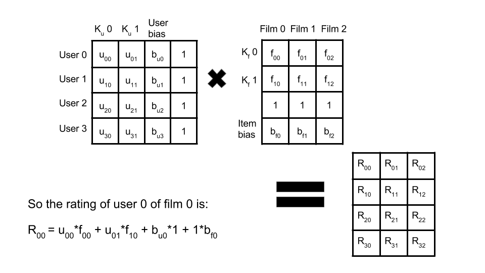
The equation for the rating of user 0 of film 0 is shown: this demonstrates how the variables of the user and the movie interact to predict this rating. $u_{00}$ and $u_{01}$ are two variables for that user, and $f_{00}$ and $f_{01}$ .

It’s possible the two user variables might represent the user’s age and location (e.g. a large number for very urban location, small for rural), and the movie variables might encode representations of the movie genre e.g. one variable may relate to crime thriller and the other to comedy. Then, if there existed a trend for older people who live in urban areas to like comedic crime movies this method would predict a high rating.

Finally, because not all users assign ratings in the same way (some users may be harsher raters and never give a movie above a 4 etc) we want to take account of this “bias” by adding a column of user bias values. A similar effect may be present for different types of movies (an epic movie may naturally garner higher ratings than a low budget rom-com) so we take account of this with an equivalent row of movie bias values. A corresponding column/row of ones is added to the user/movie matrix so the biases are treated separately (as shown in the equation).

A quick reminder of the data set is shown below

names = ['user_id', 'movie_id', 'rating', 'timestamp']
user_item_ratings = pd.read_csv('u.data', sep='\t', names=names)
user_item_ratings.head()

	user_id	movie_id	rating	timestamp
0	196	242	3	881250949
1	186	302	3	891717742
2	22	377	1	878887116
3	244	51	2	880606923
4	166	346	1	886397596

# Summary numbers

num_ratings = len(user_item_ratings)
num_users = len(user_item_ratings['user_id'].unique())
num_movies = len(user_item_ratings['movie_id'].unique())
mean_rating_overall = user_item_ratings['rating'].mean()

mean_rating_per_user = user_item_ratings.groupby('user_id').apply(lambda x: 
                                                                  x['rating'].mean())

mean_rating_per_movie = user_item_ratings.groupby('movie_id').apply(lambda x: 
                                                                  x['rating'].mean())

fig = plt.figure(figsize=(10,10))
ax = fig.add_subplot(111)
ax.hist(mean_rating_per_user, label='per user')
ax.hist(mean_rating_per_movie, alpha=0.5, label='per movie')
ax.set_xlabel('mean rating given', fontsize=24)
handles, labels = ax.get_legend_handles_labels()
ax.legend(handles, labels, fontsize=20, loc='upper left')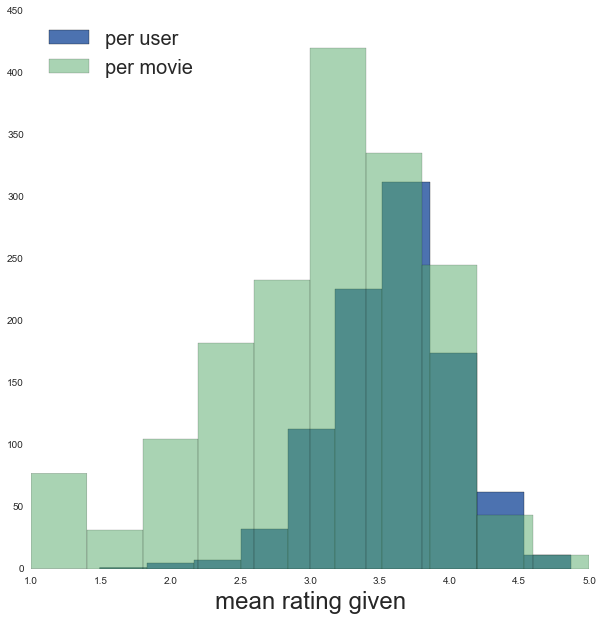

png

The algorithm

The function below details the algorithm that learns the hidden factors via gradient descent minimizing the cost function, which is basically the regularized sum of the differences squared between the predicted and true ratings.

The most important arguments are (beside the actual training_set data):

d: the number of hidden variables to learn
lam: the amount of regularisation (0=no regularisation)
lr: the learning rate of the gradient descent

def matrix_factorisation(training_set, d=2, lam=0, lr=0.01, mode='factors',
                         max_iter=1000, convergence=1e-6):
    """Matrix factorisation function
    
       @param training_set    training set rating data: 
                               'rating', 'user_id', 'movie_id' columns
       @param d               number of latent features to learn
       @param lam             regularisation parameter (lam=0 is no regularization)
       @param lr              learning rate of optimizer
       @param mode            if 'factors': learn factors without user/movie bias
                              if 'user_bias': learn user bias
                              if 'movie_bias': learn movie bias
                              if a tuple of (user_bias, movie_bias): learn factors with bias
       @param max_iter        maximum number of iterations
       @param convergence     algorithm converges when Delta-cost<convergence
    """
    
    
    ## EXTRACT DATA
    ratings = training_set['rating'].values
    mean_rating_overall = training_set['rating'].mean()


    # subtract 1 so user_id and movie_id align with zero-indexing
    userid_training = training_set['user_id'].values - 1   
    moveid_training = training_set['movie_id'].values - 1

    # number of ratings, unique users and unique movies in the training set
    num_training = len(training_set)
    num_users = len(training_set['user_id'].unique())
    num_movies = len(training_set['movie_id'].unique())
    
    
    ### THE SET UP

    # latent matrices to learn
    if mode=='factors':
        
        # simply initalise everything to 0.1
        W = tf.Variable(tf.mul(tf.ones([num_users, d]), 0.1), name='W')
        H = tf.Variable(tf.mul(tf.ones([d, num_movies]), 0.1), name='H')
        
        # regularizer
        regularizer = tf.mul(tf.add(tf.reduce_sum(tf.square(W)), 
                                    tf.reduce_sum(tf.square(H))), 
                            lam, name="regularizer")
        
    elif mode=='user_bias':
        
        # W is column of 0.1
        W = tf.Variable(tf.mul(tf.ones([num_users, 1]), 0.1), name='W')
        
        # row of 1's for H
        H = tf.ones((1, num_movies), name="H")
        
        # regularizer
        regularizer = tf.mul(tf.reduce_sum(tf.square(W)), lam, name="regularize")
        
    elif mode=='movie_bias':
        
        # column of 1's for W
        W = tf.ones((num_users, 1), name="W")
        
        # H is row of 0.1
        H = tf.Variable(tf.mul(tf.ones([1, num_movies]), 0.1), name='H')
        
        # regularizer
        regularizer = tf.mul(tf.reduce_sum(tf.square(H)), lam, name="regularize")
        
    elif isinstance(mode, tuple):   
        
        # simply initalise everything to 0.1
        Wtmp = tf.Variable(tf.mul(tf.ones([num_users, d]), 0.1), name='W')
        Htmp = tf.Variable(tf.mul(tf.ones([d, num_movies]), 0.1), name='H')
        

        # To W (user) matrix add column of user bias and column of 1's
        W = tf.concat(1, [Wtmp, tf.convert_to_tensor(mode[0], 
                                                     #dtype=float32, 
                                                     name="user_bias"), 
                                tf.ones((num_users,1), 
                                        #dtype=float32, 
                                        name="movie_ones")])

        # To H (movie) matrix add row of movie bias and row of 1's
        H = tf.concat(0, [Htmp, 
                          tf.ones((1, num_movies), 
                                  name="user_bias_ones"), 
                                  #dtype=float32), 
                          tf.convert_to_tensor(mode[1], 
                                               #dtype=float32, 
                                               name="movie_bias")])

        # regularizer
        regularizer = tf.mul(tf.add(tf.reduce_sum(tf.square(W)), 
                                    tf.reduce_sum(tf.square(H))), 
                             lam, name="regularizer")



    # Multiply the factors to get our result as a dense matrix
    # Shape is n_users * n_movies
    ratings_matrix = tf.matmul(W, H)


    # Reshape ratings matrix into sparse representation including only rated movies
    ratings_sparse_matrix = tf.gather(params=tf.reshape(ratings_matrix, [-1]), 
                    indices=userid_training*tf.shape(ratings_matrix)[1] + moveid_training, 
                    name="predicted_relative_ratings")


    # rating_pred - rating_truth
    diff_rating = tf.sub(tf.add(ratings_sparse_matrix, mean_rating_overall, name="add_mean"), 
                        ratings, name="raw_rating_diff")


    # sum((rating_pred - rating_truth)^2)
    unreg_cost = tf.reduce_sum(tf.square(diff_rating, name="squared_diff"), 
                               name="sum_squared_error")


    # root-mean-square-error
    rmse = tf.sqrt(unreg_cost/float(num_training)) 


    # cost function: unregularised cost + regularisation terms
    training_cost = tf.div(tf.add(unreg_cost, regularizer), num_training*2., 
                           name="cost_func_training")


    # cost function optimisation
    optimizer = tf.train.GradientDescentOptimizer(learning_rate=lr)
    train_step = optimizer.minimize(training_cost)


    ### THE EXECUTION
    sess = tf.Session()
    sess.run(tf.initialize_all_variables())

    
    
    # Initialise all the variable we have created
    init = tf.initialize_all_variables()

    last_cost = 0
    costs = []
    for i in range(max_iter):

        _, current_cost = sess.run([train_step, training_cost])
        costs.append(current_cost)


        # print Delta-cost ten times during iterations
        if i%int(max_iter/10.)==0:
            print "Iteration", i+1, "current cost =", current_cost,
            print "Delta-cost =", abs(last_cost - current_cost)


        if abs(last_cost - current_cost) < convergence:
            print "Converged at iteration", i+1
            print last_cost, current_cost
            break

        last_cost = current_cost

    # Evaluate performance
    end_rmse_training = rmse.eval(session=sess) 

    end_W = W.eval(session=sess)
    end_H = H.eval(session=sess)

    ratings_predictions = ratings_sparse_matrix.eval(session=sess) 

    sess.close()
    

    return end_W, end_H, end_rmse_training, ratings_predictions, mean_rating_overall, costs

The training set

As a first exploration of this method we just use the entire 10,000 ratings to train with.

In practice not only would you use a subset to train with but you would also set asside a cross-validation set to learn the optimum number of hidden variables to learn and the optimum regularisation to use.

training_set = user_item_ratings

Not including user or item bias

To begin we see what kind of precision we get when we ignore the user and item biases. Here we set there to be 100 hidden variables to learn (100 user ones + 100 movie ones) and set the learning rate to 10 (for fast convergence).

results = matrix_factorisation(training_set, d=100, lr=10.)

end_W_no_bias = results[0]
end_H_no_bias = results[1]
end_rmse_no_bias = results[2]
ratings_predictions_no_bias = results[3] 
mean_rating_overall = results[4]
costs = results[5]

print "Final RMSE =", end_rmse_no_bias

Iteration 1 current cost = 1.13354 Delta-cost = 1.1335362196
Iteration 101 current cost = 0.572312 Delta-cost = 0.000516891
Iteration 201 current cost = 0.548027 Delta-cost = 0.000113606
Iteration 301 current cost = 0.540612 Delta-cost = 4.91738e-05
Iteration 401 current cost = 0.536911 Delta-cost = 2.85506e-05
Iteration 501 current cost = 0.534622 Delta-cost = 1.87159e-05
Iteration 601 current cost = 0.533034 Delta-cost = 1.32322e-05
Iteration 701 current cost = 0.531851 Delta-cost = 1.06096e-05
Iteration 801 current cost = 0.530925 Delta-cost = 8.10623e-06
Iteration 901 current cost = 0.530173 Delta-cost = 6.79493e-06
Final RMSE = 1.02912

fig = plt.figure(figsize=(10,10))
ax = fig.add_subplot(111)
ax.plot(costs)
ax.set_xlabel('iteration', fontsize=24)
ax.set_ylabel('cost function', fontsize=24)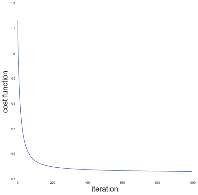

png

bins = [0.5, 1.5, 2.5, 3.5, 4.5, 5.5]

fig = plt.figure(figsize=(10,10))
ax = fig.add_subplot(111)
ax.hist(ratings_predictions_no_bias + mean_rating_overall, bins=bins, 
        label='predicted')
ax.hist(training_set['rating'].values, alpha=0.5, bins=bins, 
        label='true ratings')
handles, labels = ax.get_legend_handles_labels()
ax.legend(handles, labels, loc='upper left', fontsize=20)
ax.set_xlabel('rating', fontsize=20)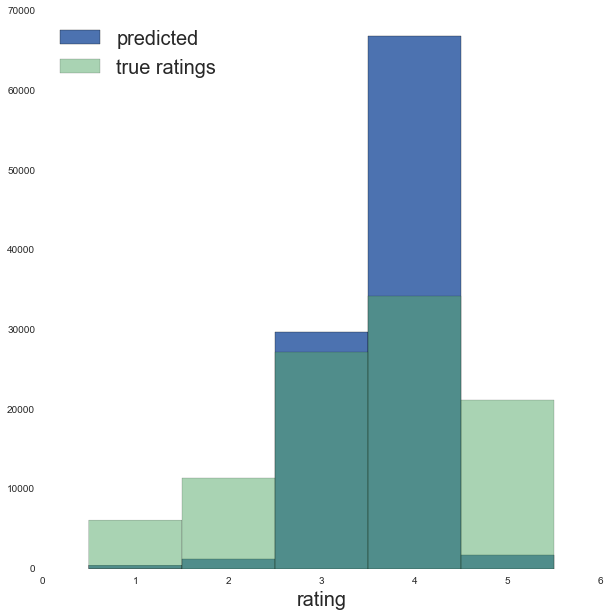

png

The results are ok, the root-mean-square-error is about +/- 1 rating. However we can see from the distribution of ratings the predictions are ending up too tightly clustered around the mean overall rating

Learn user bias alone

While we learn the column of user bias we can also see how well a having only a single column of user bias can predict the ratings.

Note that now mode is set to be user_bias

results = matrix_factorisation(training_set, d=100, lr=10., mode='user_bias')

W_user_bias = results[0]
H_user_bias = results[1]
end_rmse_user_bias = results[2]
ratings_predictions_user_bias = results[3] 
mean_rating_overall = results[4]
costs = results[5]

print "Final RMSE =", end_rmse_user_bias

Iteration 1 current cost = 0.638533 Delta-cost = 0.638532996178
Iteration 101 current cost = 0.542808 Delta-cost = 0.000134468
Iteration 201 current cost = 0.535901 Delta-cost = 3.67165e-05
Iteration 301 current cost = 0.533597 Delta-cost = 1.54972e-05
Iteration 401 current cost = 0.53255 Delta-cost = 7.21216e-06
Iteration 501 current cost = 0.53201 Delta-cost = 3.8743e-06
Iteration 601 current cost = 0.531713 Delta-cost = 2.26498e-06
Iteration 701 current cost = 0.531543 Delta-cost = 1.13249e-06
Converged at iteration 704
0.53154 0.531539
Final RMSE = 1.03106

bins = [0.5, 1.5, 2.5, 3.5, 4.5, 5.5]

fig = plt.figure(figsize=(10,10))
ax = fig.add_subplot(111)
ax.hist(ratings_predictions_user_bias + mean_rating_overall, bins=bins, 
        label='predicted')
ax.hist(training_set['rating'].values, alpha=0.5, bins=bins, 
        label='true ratings')
handles, labels = ax.get_legend_handles_labels()
ax.legend(handles, labels, loc='upper left', fontsize=20)
ax.set_xlabel('rating', fontsize=20)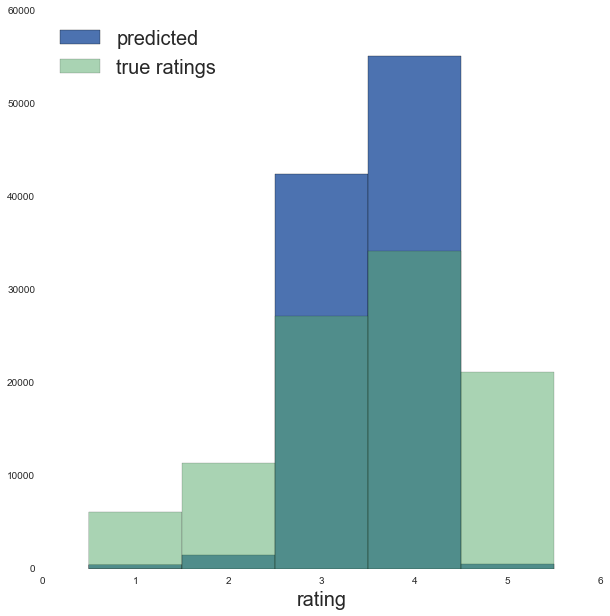

png

The performance is very similar to running without bias but with 100 hidden variables. However the predictions look more clustered around the mean rating than before.

Learn movie bias alone

Repeating the same thing, but now for the movie bias.

Note that now mode is set to be movie_bias

results = matrix_factorisation(training_set, d=100, lr=10., mode='movie_bias')

W_movie_bias = results[0]
H_movie_bias = results[1]
end_rmse_movie_bias = results[2]
ratings_predictions_movie_bias = results[3] 
mean_rating_overall = results[4]
costs = results[5]

print "Final RMSE =", end_rmse_movie_bias

Iteration 1 current cost = 0.638533 Delta-cost = 0.638532996178
Iteration 101 current cost = 0.547283 Delta-cost = 0.000288308
Iteration 201 current cost = 0.529536 Delta-cost = 0.000110269
Iteration 301 current cost = 0.521484 Delta-cost = 5.93066e-05
Iteration 401 current cost = 0.516879 Delta-cost = 3.67761e-05
Iteration 501 current cost = 0.513903 Delta-cost = 2.42591e-05
Iteration 601 current cost = 0.511821 Delta-cost = 1.78218e-05
Iteration 701 current cost = 0.510283 Delta-cost = 1.33514e-05
Iteration 801 current cost = 0.509098 Delta-cost = 1.055e-05
Iteration 901 current cost = 0.508156 Delta-cost = 8.70228e-06
Final RMSE = 1.00736

bins = [0.5, 1.5, 2.5, 3.5, 4.5, 5.5]

fig = plt.figure(figsize=(10,10))
ax = fig.add_subplot(111)
ax.hist(ratings_predictions_movie_bias + mean_rating_overall, bins=bins, 
        label='predicted')
ax.hist(training_set['rating'].values, alpha=0.5, bins=bins, 
        label='true ratings')
handles, labels = ax.get_legend_handles_labels()
ax.legend(handles, labels, loc='upper left', fontsize=20)
ax.set_xlabel('rating', fontsize=20)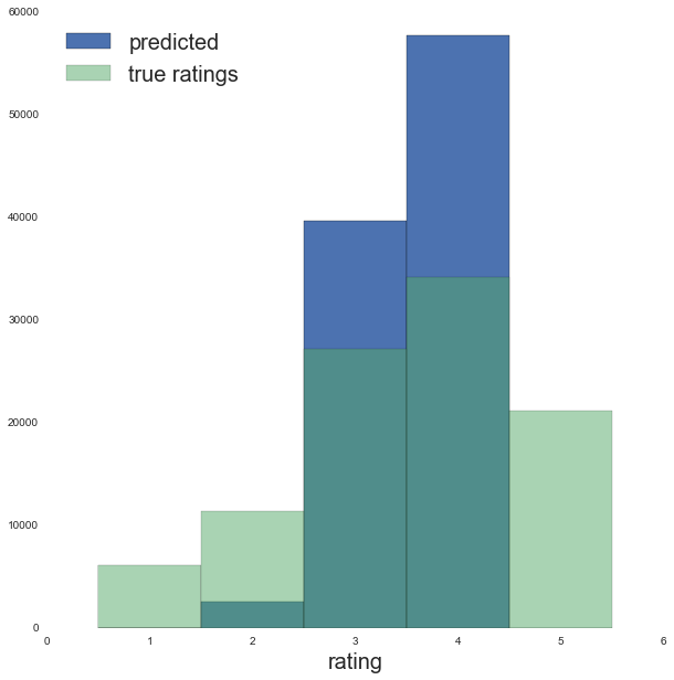

png

So far the performance is best when just including the movie bias!

Including bias

Note that now mode is set to be a tuple of the learned user bias matrix and the learned movie bias matrix.

results = matrix_factorisation(training_set, d=100, lr=10., 
                               mode=(W_user_bias, H_movie_bias))

W_full = results[0]
H_full = results[1]
end_rmse_full = results[2]
ratings_predictions_full = results[3] 
mean_rating_overall = results[4]
costs = results[5]

print "Final RMSE =", end_rmse_full

Iteration 1 current cost = 0.958202 Delta-cost = 0.9582015872
Iteration 101 current cost = 0.469477 Delta-cost = 0.000476152
Iteration 201 current cost = 0.445877 Delta-cost = 0.000118017
Iteration 301 current cost = 0.438018 Delta-cost = 5.33164e-05
Iteration 401 current cost = 0.433981 Delta-cost = 3.10242e-05
Iteration 501 current cost = 0.431411 Delta-cost = 2.18451e-05
Iteration 601 current cost = 0.429543 Delta-cost = 1.66595e-05
Iteration 701 current cost = 0.428053 Delta-cost = 1.33812e-05
Iteration 801 current cost = 0.426783 Delta-cost = 1.20699e-05
Iteration 901 current cost = 0.42565 Delta-cost = 1.06394e-05
Final RMSE = 0.921525

bins = [0.5, 1.5, 2.5, 3.5, 4.5, 5.5]

fig = plt.figure(figsize=(10,10))
ax = fig.add_subplot(111)
ax.hist(ratings_predictions_full + mean_rating_overall, bins=bins, 
        label='predicted')
ax.hist(training_set['rating'].values, alpha=0.5, bins=bins, 
        label='true ratings')
handles, labels = ax.get_legend_handles_labels()
ax.legend(handles, labels, loc='upper left', fontsize=20)
ax.set_xlabel('rating', fontsize=20)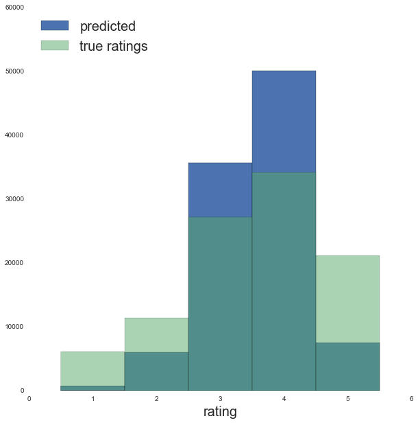

png

drating = abs(np.round(training_set['rating'] - 
              (ratings_predictions_full + mean_rating_overall)))
    

hist_data = ax.hist(drating, bins=[-0.5, 0.5, 1.5, 2.5, 3.5, 4.5, 5.5])

fig = plt.figure(figsize=(10,10))
ax = fig.add_subplot(111)
ax.bar(np.arange(0, 6, 1), hist_data[0]/float(len(drating)), width=0.3)
ax.set_xlabel('$\Delta$-rating from true rating', fontsize=24)
ax.set_ylabel('percentage of predicted ratings', fontsize=24)
ax.set_xlim([0,5])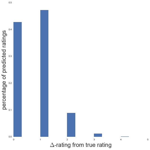

png

43% of predictions were correct, and 47% were only 1 rating off, so 10% of predictions were 2 or more ratings off. I don’t know how “good” these results actually are for typical implementations of this method, though a quick google search showed RMSE’s that were comparable to ~0.9 (result achieved here is 0.92). However, if you are within 1 rating (out of a total of 5) 90% of the time, then I think 90% of the time you definitely manage to discriminate between whether a user “likes” or “dislikes” a movie.