Movie Lens!
The MovieLens data set
This is a classic data set that is used by people who want to try out recommender system approaches. It was set up in 1997 by a group at the University of Minnesota who wanted to gather research data on personalised recommendations.
We have the following three tables:
- the ratings users gave to movies
- data on the users (age, gender, occupation, zip code)
- data on the movies (title, release data, genre(s))
In this version of the data set we have 100,000 ratings of nearly 1700 movies from nearly 1000 users.
User ratings for movies
This table is the ‘meat’ required for any recommender approach: the actual ratings
names = ['user_id', 'movie_id', 'rating', 'timestamp']
user_item_ratings = pd.read_csv('u.data', sep='\t', names=names)
user_item_ratings.head()| user_id | movie_id | rating | timestamp | |
|---|---|---|---|---|
| 0 | 196 | 242 | 3 | 881250949 |
| 1 | 186 | 302 | 3 | 891717742 |
| 2 | 22 | 377 | 1 | 878887116 |
| 3 | 244 | 51 | 2 | 880606923 |
| 4 | 166 | 346 | 1 | 886397596 |
number_of_unique_users = len(user_item_ratings['user_id'].unique())
number_of_unique_movies = len(user_item_ratings['movie_id'].unique())
number_of_ratings = len(user_item_ratings)
print "Number of unique users =", number_of_unique_users
print "Number of unique movies =", number_of_unique_movies
print "Number of ratings =", number_of_ratings
Number of unique users = 943
Number of unique movies = 1682
Number of ratings = 100000
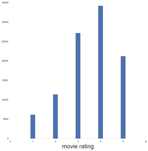
fig = plt.figure(figsize=(10,10))
ax = fig.add_subplot(111)
ax.hist(user_item_ratings['rating'], bins=[0.9, 1.1, 1.9, 2.1, 2.9, 3.1, 3.9, 4.1, 4.9, 5.1])
ax.set_xlabel('movie rating', fontsize=24)

mean_rating = user_item_ratings['rating'].mean()
print "Mean rating =", mean_rating
Mean rating = 3.52986
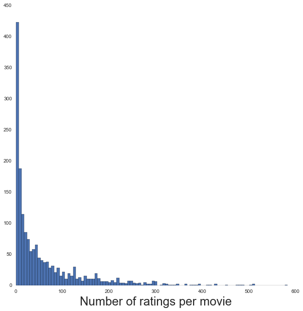
# Number of ratings per movie
num_ratings_per_movie = user_item_ratings['movie_id'].value_counts().values

fig = plt.figure(figsize=(10,10))
ax = fig.add_subplot(111)
ax.hist(num_ratings_per_movie, 100)
ax.set_xlabel('Number of ratings per movie', fontsize=24)

print len(np.where(num_ratings_per_movie<2)[0]), "movies were rated by only 1 user"
141 movies were rated by only 1 user
# mean ratings from each user
mean_rating_of_user = user_item_ratings.groupby('user_id').apply(lambda x:
                                                                 x['rating'].mean())

fig = plt.figure(figsize=(10,10))
ax = fig.add_subplot(111)
ax.hist(mean_rating_of_user)
ax.set_xlabel('mean rating given by each user', fontsize=24)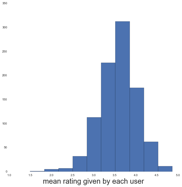
Movie data
names = ['movie_id', 'movie_title', 'release_date', 'video_release_date',
         'IMDb_URL' , 'unknown' , 'Action' , 'Adventure' , 'Animation' ,
         'Children' , 'Comedy' , 'Crime' , 'Documentary' , 'Drama' , 'Fantasy' ,
         'Film-Noir' , 'Horror' , 'Musical' , 'Mystery' , 'Romance' , 'Sci-Fi' ,
         'Thriller' , 'War' , 'Western']
movies = pd.read_csv('u.item', sep='|', names=names).set_index('movie_id')
movies.head()| movie_title | release_date | video_release_date | IMDb_URL | unknown | Action | Adventure | Animation | Children | Comedy | ... | Fantasy | Film-Noir | Horror | Musical | Mystery | Romance | Sci-Fi | Thriller | War | Western | |
|---|---|---|---|---|---|---|---|---|---|---|---|---|---|---|---|---|---|---|---|---|---|
| movie_id | |||||||||||||||||||||
| 1 | Toy Story (1995) | 01-Jan-1995 | NaN | http://us.imdb.com/M/title-exact?Toy%20Story%2... | 0 | 0 | 0 | 1 | 1 | 1 | ... | 0 | 0 | 0 | 0 | 0 | 0 | 0 | 0 | 0 | 0 |
| 2 | GoldenEye (1995) | 01-Jan-1995 | NaN | http://us.imdb.com/M/title-exact?GoldenEye%20(... | 0 | 1 | 1 | 0 | 0 | 0 | ... | 0 | 0 | 0 | 0 | 0 | 0 | 0 | 1 | 0 | 0 |
| 3 | Four Rooms (1995) | 01-Jan-1995 | NaN | http://us.imdb.com/M/title-exact?Four%20Rooms%... | 0 | 0 | 0 | 0 | 0 | 0 | ... | 0 | 0 | 0 | 0 | 0 | 0 | 0 | 1 | 0 | 0 |
| 4 | Get Shorty (1995) | 01-Jan-1995 | NaN | http://us.imdb.com/M/title-exact?Get%20Shorty%... | 0 | 1 | 0 | 0 | 0 | 1 | ... | 0 | 0 | 0 | 0 | 0 | 0 | 0 | 0 | 0 | 0 |
| 5 | Copycat (1995) | 01-Jan-1995 | NaN | http://us.imdb.com/M/title-exact?Copycat%20(1995) | 0 | 0 | 0 | 0 | 0 | 0 | ... | 0 | 0 | 0 | 0 | 0 | 0 | 0 | 1 | 0 | 0 |
5 rows × 23 columns
genres = ['unknown' , 'Action' , 'Adventure' , 'Animation' ,
         'Children' , 'Comedy' , 'Crime' , 'Documentary' , 'Drama' , 'Fantasy' ,
         'Film-Noir' , 'Horror' , 'Musical' , 'Mystery' , 'Romance' , 'Sci-Fi' ,
         'Thriller' , 'War' , 'Western']

fig = plt.figure(figsize=(10,10))
ax = fig.add_subplot(111)
movies[genres].sum().sort_values().plot(kind='barh', stacked=False, ax=ax)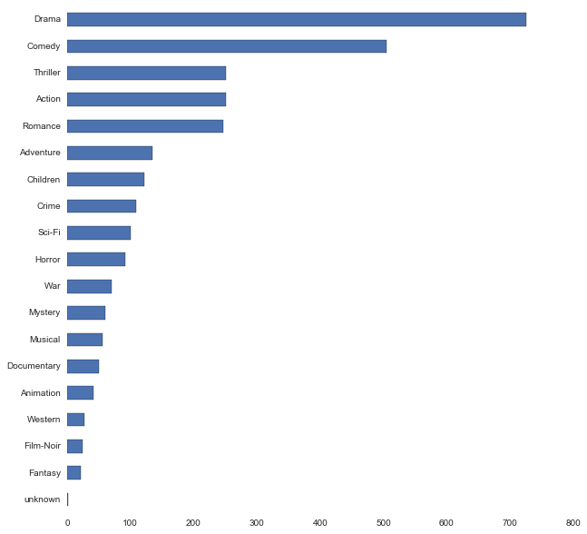
Users
names = ['user_id', 'age', 'gender', 'occupation', 'zip_code']
users = pd.read_csv('u.user', sep='|', names=names).set_index('user_id')
users.head()| age | gender | occupation | zip_code | |
|---|---|---|---|---|
| user_id | ||||
| 1 | 24 | M | technician | 85711 |
| 2 | 53 | F | other | 94043 |
| 3 | 23 | M | writer | 32067 |
| 4 | 24 | M | technician | 43537 |
| 5 | 33 | F | other | 15213 |
fig = plt.figure(figsize=(10,8))
ax = fig.add_subplot(111)
users['gender'].value_counts().plot(kind='barh', stacked=False, ax=ax)
ax.set_yticklabels(['Male', 'Female'], fontsize=20)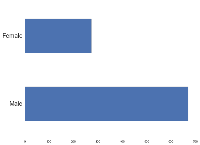
grouped_by_gender = users.groupby(["occupation","gender"]).size().unstack(
                           "gender").fillna(0)

frac_gender = grouped_by_gender.divide(grouped_by_gender.sum(axis=1), axis='rows')


fig = plt.figure(figsize=(10,8))
ax = fig.add_subplot(111)
frac_gender.sort_values('M').plot(kind='barh', stacked=False, ax=ax,
                       color=sns.color_palette('hls'))
ax.legend(fontsize=24, loc='lower right')
ax.set_ylabel('')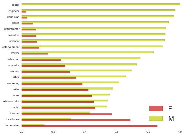
def outline_boxes_with_color(bp, col, color):
    """Change all lines on boxplot, the box outline, the median line, the whiskers and
       the caps on the ends to be 'color'

       @param bp       handle of boxplot
       @param col      column
       @param color    color to change lines to
    """

    plt.setp(bp[col]['boxes'], color=color)
    plt.setp(bp[col]['whiskers'], color=color)
    plt.setp(bp[col]['medians'], color=color)
    plt.setp(bp[col]['caps'], color=color)

fig = plt.figure(figsize=(10,10))
ax = fig.add_subplot(111)
col = 'age'
bp = users.boxplot(column=[col], return_type='dict',
                         by='occupation', ax=ax)
outline_boxes_with_color(bp, col, 'black')
ax.set_xlabel('', fontsize=24)
ax.set_ylabel('Age', fontsize=24)
ax.set_title('')
plt.xticks(rotation='vertical', fontsize=18)
fig.suptitle('')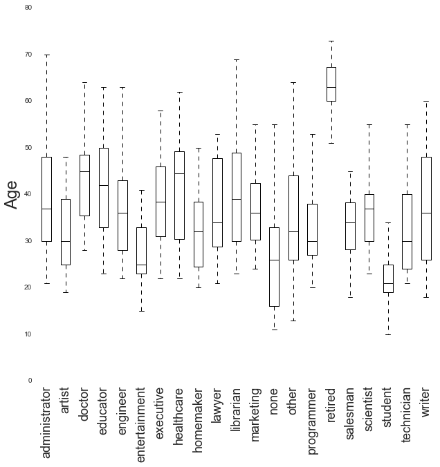
User-item matrix
ratings_matrix = np.zeros((number_of_unique_users, number_of_unique_movies))

for index, row in user_item_ratings.iterrows():
    user_id = row['user_id']
    movie_id = row['movie_id']
    rating = row['rating']

    ratings_matrix[user_id-1, movie_id-1] = rating
sparsity = 100.*float(len(ratings_matrix.nonzero()[0]))/ratings_matrix.size
print 'Sparsity of the user-item matrix ={0:4.1f}%'.format(sparsity)Sparsity of the user-item matrix = 6.3%
Step 0: Most basic recommendation
Predict rating to always be the mean movie rating! This is the baseline we seek to improve upon.
rmse_benchmark = np.sqrt(pow(user_item_ratings['rating']-mean_rating, 2).mean())
print "Maximum root-mean-square error = {:4.2f}".format(rmse_benchmark)
Maximum root-mean-square error = 1.13
Step 1: Rating prediction based upon user-user similarity
We define “similarity” using the cosine similarity metric. Imagining each user’s set of ratings as a vector, the cosine similarity of two users is simply the cosine of the angle between their two vectors. This is given by the dot product of the two vectors divided by their magnitudes:
And for ease i’ll simply do a ‘leave one out’ approach: for every user I will use the other users’ ratings to predict that user’s ratings, and then calculate an overall root-mean-square-error on those predictions.
The code below is also slow because it’s not taking full advantage of matrix operations, but THIS CODE IS FOR ILLUSTRATION ONLY!
from sklearn.metrics.pairwise import cosine_similarity

# Calculate the similarity score between users
user_user_similarity = cosine_similarity(ratings_matrix)
user_user_similarity.shape
(943, 943)
Predict a rating as exactly the rating given by the most similar user
sqdiffs = 0
num_preds = 0
cnt_no_other_ratings = 0

# for each user
for user_i, u in enumerate(ratings_matrix):

    # movies user HAS rated
    i_rated = np.where(u>0)[0]

    # for each rated movie: find most similar user who HAS ALSO rated this movie
    for imovie in i_rated:

        # all users that have rated imovie (includes user of interest)
        i_has_rated = np.where(ratings_matrix[:, imovie]>0)[0]

        # remove the current user
        iremove = np.argmin(abs(i_has_rated - user_i))
        i_others_have_rated = np.delete(i_has_rated, iremove)


        # find most similar user that has also rated imovie to current user
        try:
            i_most_sim = np.argmax(user_user_similarity[user_i, i_others_have_rated])
        except:
            cnt_no_other_ratings += 1
            continue

        # prediction error
        predicted_rating = ratings_matrix[i_others_have_rated[i_most_sim], imovie]
        actual_rating = ratings_matrix[user_i, imovie]

        sqdiffs += pow(predicted_rating-actual_rating, 2.)
        num_preds += 1


rmse_cossim = np.sqrt(sqdiffs/num_preds)

print "Failed to make", cnt_no_other_ratings ,"predictions"
print "Number of predictions made =", num_preds
print "Root mean square error =", rmse_cossim
Failed to make 141 predictions
Number of predictions made = 99859
Root mean square error = 1.30217928718
Erm, it got worse! Let’s try something more sensible. (The failed predictions occur because that movie was only rated by a single user.)
Predict a rating as the weighted mean of all ratings
Weighted by the user similarities …
sqdiffs = 0
num_preds = 0

# to protect against divide by zero issues
eps = 1e-6

cnt_no_sims = 0

# for each user
for user_i, u in enumerate(ratings_matrix):

    # movies user HAS rated
    i_rated = np.where(u>0)[0]

    # for each rated movie: find users who HAVE ALSO rated this movie
    for imovie in i_rated:

        # all users that have rated imovie (includes user of interest)
        i_has_rated = np.where(ratings_matrix[:, imovie]>0)[0]

        # remove the current user
        iremove = np.argmin(abs(i_has_rated - user_i))
        i_others_have_rated = np.delete(i_has_rated, iremove)


        # rating is weighted sum of all ratings, weights are cosine sims
        ratings = ratings_matrix[i_others_have_rated, imovie]
        sims = user_user_similarity[user_i, i_others_have_rated]

        norm = np.sum(sims)
        if norm==0:
            cnt_no_sims += 1
            norm = eps

        predicted_rating = np.sum(ratings*sims)/norm


        # prediction error
        actual_rating = ratings_matrix[user_i, imovie]

        sqdiffs += pow(predicted_rating-actual_rating, 2.)
        num_preds += 1


rmse_cossim = np.sqrt(sqdiffs/num_preds)

print cnt_no_sims, "movies had only one user rating"
print "Number of predictions made =", num_preds
print "Root mean square error =", rmse_cossim
141 movies had only one user rating
Number of predictions made = 100000
Root mean square error = 1.01584998447
It improved! Can we do any better by only counting the top most similar users in the weighted sum?
def rmse_topN(topN):
    """Return the root-mean-square-error given value topN
       for using the 'top N' most similar users in predicting
       the rating
    """

    sqdiffs = 0
    num_preds = 0

    # to protect against divide by zero issues
    eps = 1e-6

    cnt_no_sims = 0

    # for each user
    for user_i, u in enumerate(ratings_matrix):

        # movies user HAS rated
        i_rated = np.where(u>0)[0]

        # for each rated movie:
        for imovie in i_rated:

            # all users that have rated imovie (includes user of interest)
            i_has_rated = np.where(ratings_matrix[:, imovie]>0)[0]

            # remove the current user
            iremove = np.argmin(abs(i_has_rated - user_i))
            i_others_have_rated = np.delete(i_has_rated, iremove)


            # rating is weighted sum of all ratings, weights are cosine sims
            ratings = ratings_matrix[i_others_have_rated, imovie]
            sims = user_user_similarity[user_i, i_others_have_rated]

            # only want top n sims
            most_sim_users = sims[np.argsort(sims*-1)][:topN]
            most_sim_ratings = ratings[np.argsort(sims*-1)][:topN]

    #         if user_i == 0:
    #             break

            norm = np.sum(most_sim_users)
            if norm==0:
                cnt_no_sims += 1
                norm = eps

            predicted_rating = np.sum(most_sim_ratings*most_sim_users)/norm


            # prediction error
            actual_rating = ratings_matrix[user_i, imovie]

            sqdiffs += pow(predicted_rating-actual_rating, 2.)
            num_preds += 1

    #     if user_i == 0:
    #         break

    rmse_cossim = np.sqrt(sqdiffs/num_preds)

    print "Using top", topN , "most similar users to predict rating"
    print "Number of predictions made =", num_preds
    print "Root mean square error =", rmse_cossim , '\n'
    return rmse_cossim

topN_trials = [2, 10, 25, 50, 75, 100, 300]
rmse_results = []
for topN in topN_trials:
    rmse_results.append(rmse_topN(topN))
Using top 2 most similar users to predict rating
Number of predictions made = 100000
Root mean square error = 1.14548307354
Using top 10 most similar users to predict rating
Number of predictions made = 100000
Root mean square error = 1.01567130006
Using top 25 most similar users to predict rating
Number of predictions made = 100000
Root mean square error = 1.0023325746
Using top 50 most similar users to predict rating
Number of predictions made = 100000
Root mean square error = 1.0039703331
Using top 75 most similar users to predict rating
Number of predictions made = 100000
Root mean square error = 1.00673516576
Using top 100 most similar users to predict rating
Number of predictions made = 100000
Root mean square error = 1.00894503162
Using top 300 most similar users to predict rating
Number of predictions made = 100000
Root mean square error = 1.01523721106
fig = plt.figure(figsize=(10,10))
ax = fig.add_subplot(111)
ax.plot(topN_trials, rmse_results, label='using top N')
xlims = ax.get_xlim()
ax.plot(xlims, [rmse_benchmark, rmse_benchmark], color='black',
        linestyle='dotted', label='benchmark')
ax.plot(xlims, [rmse_cossim, rmse_cossim], color='blue', linestyle='dotted',
        label='using all')

ax.set_xlabel('use top N most similar users', fontsize=24)
ax.set_ylabel('RMSE', fontsize=24)
handles, labels = ax.get_legend_handles_labels()
ax.legend(handles, labels, fontsize=20)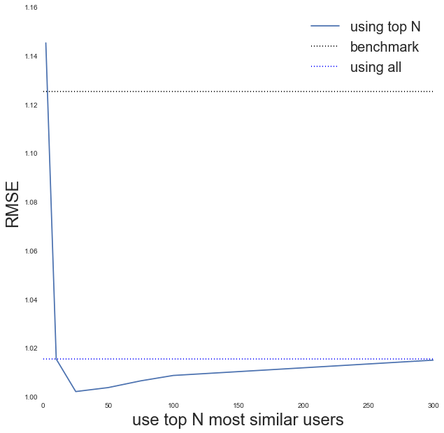
Yes it improves if we use top users, with looking like it gives the best improvement.
Step 2: item-item similarity
We can do exactly the same process for items instead of users; this time treating an item as a vector of ratings and calculate a similarity between two items in the same manner using cosine similarity.
# Calculate the similarity score between ITEMS: note the transpose
item_item_similarity = cosine_similarity(ratings_matrix.T)
item_item_similarity.shape
(1682, 1682)
def rmse_topN_items(topN):
    """Return the root-mean-square-error given value topN
       for using the 'top N' most similar ITEMS in predicting
       the rating
    """

    sqdiffs = 0
    num_preds = 0

    # to protect against divide by zero issues
    eps = 1e-6

    cnt_no_sims = 0

    # for each item
    for item_i, u in enumerate(ratings_matrix.T):

        # users item HAS ratings by
        i_rated = np.where(u>0)[0]

        # for each user that rated:
        for iuser in i_rated:

            # all movies that have been rated by iuser
            i_has_rated = np.where(ratings_matrix[iuser, :]>0)[0]

            # remove the current movie
            iremove = np.argmin(abs(i_has_rated - item_i))
            i_others_have_rated = np.delete(i_has_rated, iremove)


            # rating is weighted sum of all ratings, weights are cosine sims
            ratings = ratings_matrix[iuser, i_others_have_rated]
            sims = item_item_similarity[i_others_have_rated, item_i]

            # only want top n sims
            most_sim_users = sims[np.argsort(sims*-1)][:topN]
            most_sim_ratings = ratings[np.argsort(sims*-1)][:topN]


            norm = np.sum(most_sim_users)
            if norm==0:
                cnt_no_sims += 1
                norm = eps

            predicted_rating = np.sum(most_sim_ratings*most_sim_users)/norm


            # prediction error
            actual_rating = ratings_matrix[iuser, item_i]

            sqdiffs += pow(predicted_rating-actual_rating, 2.)
            num_preds += 1


    rmse_cossim = np.sqrt(sqdiffs/num_preds)

    print "Using top", topN , "most similar movies to predict rating"
    print "Number of predictions made =", num_preds
    print "Root mean square error =", rmse_cossim , '\n'
    return rmse_cossim

topN_trials = [2, 10, 25, 50, 75, 100, 300]
rmse_item_results = []
for topN in topN_trials:
    rmse_item_results.append(rmse_topN_items(topN))
Using top 2 most similar movies to predict rating
Number of predictions made = 100000
Root mean square error = 1.0627135524
Using top 10 most similar movies to predict rating
Number of predictions made = 100000
Root mean square error = 0.959118494932
Using top 25 most similar movies to predict rating
Number of predictions made = 100000
Root mean square error = 0.965039905069
Using top 50 most similar movies to predict rating
Number of predictions made = 100000
Root mean square error = 0.980703964443
Using top 75 most similar movies to predict rating
Number of predictions made = 100000
Root mean square error = 0.989516609768
Using top 100 most similar movies to predict rating
Number of predictions made = 100000
Root mean square error = 0.995218394229
Using top 300 most similar movies to predict rating
Number of predictions made = 100000
Root mean square error = 1.01019290087
fig = plt.figure(figsize=(10,10))
ax = fig.add_subplot(111)
ax.plot(topN_trials, rmse_item_results, label='item-item')
ax.plot(topN_trials, rmse_results, label='user-user')

xlims = ax.get_xlim()
ax.plot(xlims, [rmse_benchmark, rmse_benchmark], color='black',
        linestyle='dotted', label='benchmark')

ax.set_xlabel('use top N most similar', fontsize=24)
ax.set_ylabel('RMSE', fontsize=24)
handles, labels = ax.get_legend_handles_labels()
ax.legend(handles, labels, fontsize=20)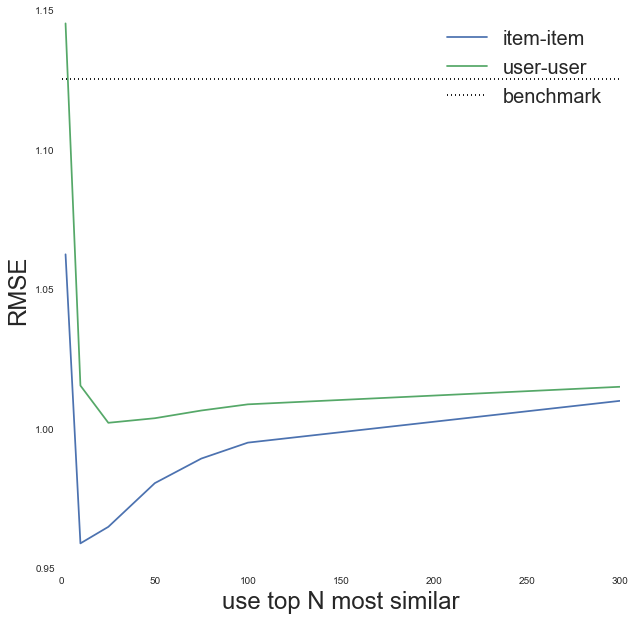
Step 3: User bias!
Not all users rate movies in the same way, so it would be more useful if the collaborative filtering looked at the relative difference between movie ratings rather than the absolute values. E.g. look at the large scatter in the distribution of the mean rating given by each user; some of this is coming from noise (some users will have only rated 10 movies), but some is also coming from the fact that some users will tend to consistently rate things higher than other users. To account fo this we simply re-define the predicted rating for user and item as:
topN = 25 # best value from before

sqdiffs = 0
num_preds = 0

# to protect against divide by zero issues
eps = 1e-6

cnt_no_sims = 0

# for each user
for user_i, u in enumerate(ratings_matrix):

    # movies user HAS rated
    i_rated = np.where(u>0)[0]

    # for each rated movie:
    for imovie in i_rated:

        # all users that have rated imovie (includes user of interest)
        i_has_rated = np.where(ratings_matrix[:, imovie]>0)[0]

        # remove the current user
        iremove = np.argmin(abs(i_has_rated - user_i))
        i_others_have_rated = np.delete(i_has_rated, iremove)


        # rating is weighted sum of all ratings, weights are cosine sims
        ratings = ratings_matrix[i_others_have_rated, imovie]
        sims = user_user_similarity[user_i, i_others_have_rated]

        # only want top n sims
        most_sim_users = sims[np.argsort(sims*-1)][:topN]
        most_sim_ratings = ratings[np.argsort(sims*-1)][:topN]

#         if user_i == 0:
#             break

        norm = np.sum(most_sim_users)
        if norm==0:
            cnt_no_sims += 1
            norm = eps

        predicted_rating = mean_rating + np.sum((most_sim_ratings-mean_rating)*most_sim_users)/norm


        # prediction error
        actual_rating = ratings_matrix[user_i, imovie]

        sqdiffs += pow(predicted_rating-actual_rating, 2.)
        num_preds += 1

#     if user_i == 0:
#         break

rmse_bias = np.sqrt(sqdiffs/num_preds)

print "Using top", topN , "most similar users to predict rating"
print "Number of predictions made =", num_preds
print "Root mean square error =", rmse_bias , '\n'
Using top 25 most similar users to predict rating
Number of predictions made = 100000
Root mean square error = 0.99968273602
It improved slightly upon no bias!
Summary
Alright! So after trying the following, predict user ’s rating of movie as being:
- the same rating as the most similar user to user who has rated movie (result=bad)
- the weighted sum of ratings by all other users who have rated movie . The weights are given by the other users’ similarities to user (result=ok)
- the weighted sum of ratings by the top k most similar users to user who have also rated movie (result=ok)
- as above, taking account of “user bias” (result=ok)
- the weighted sum of ratings for the top k most similar movies to movie (result=best)
Using the top-10 most similar items with an item-item collaborative filtering approach seems to perform the best!
To be continued …. to play with one or more of: matrix factorisation, additional features!