SGD and TensorFlow
TensorFlow
TensorFlow is literally the “flow” of “tensors”! It runs a series of computations that it represents as a graph with nodes. At each node an “Operation” occurs that requires 0 or more “Tensor”s and produces 0 or more “Tensor”s. Each “Tensor” is a structured, typed, representation of the data.
TensorFlow has many high level data types we need to understand:
- Constant: variable that does not depend on data (e.g. a mxn matrix of 3’s), a static value
- Tensor: this represents the data, the only thing passed between ops
- Variable: these record and maintain the state of the system/model
- Operation: an arbitrary operation, e.g. a function that is called on a Tensor with Variables
- Session (this is the workhorse!)
The “Session” is the thing that launches the graph that describes the computations. The “Session” provides the methods with which to perform the Operations and also places the corresponding process on to the correct device (e.g. CPU or GPU).
Setting up TensorFlow to do a computation requires two stages:
- Set up the graph
- Execute the graph
For example, if we wanted to multiply two matrices:
### THE SET UP

# This creates a Constant op that produces a 1x2 matrix: matrix1 = [2,3]
matrix1 = tf.constant([[2., 3.]])

# And now a 2x1 matrix: matrix2 = [5,1]^T
matrix2 = tf.constant([[5.],[1.]])

# This create a matmul op that takes 'matrix1' and 'matrix2' as inputs.
# And the returned value represents the result of the matrix multiplication.
product = tf.matmul(matrix1, matrix2)


### THE EXECUTION
sess = tf.Session()
result = sess.run(product)

print result
print type(result)


# Close the Session: remember to do this to release resources!
sess.close()
[[ 13.]]
<type 'numpy.ndarray'>
We see that we get returned a 1x1 numpy array equal to the multiplication of the two matrices.
We could get complicated here and go into how TensorFlow can distribute the executable operations across available compute resources, but I’m more interested in how the API works.
Stochastic Gradient Descent
I want a refresher on stochastic gradient descent, and since I’m also keen to learn how to use TensorFlow, so I’m going to follow the tutorial given here.
In usual gradient descent (see this previous post) we minimised the cost function; simultaneously updating every feature parameter using the full data set. Stochastic gradient descent however, updates using a single sample at a time, or a mini-batch of samples. It is an approximation to gradient descent on the full set of samples, and should converge to the same solution. It can be an advantage for large data sets, when the evaluation of the gradient of the cost function could become expensive, or for data sets with streaming input data.
The implementation
First step is to download the MNIST data, a database of images of handwritten digits, tagged with lables indicating the digit they represent.
import tensorflow as tf

from tensorflow.examples.tutorials.mnist import input_data

# A one-hot vector is a vector which is 0 in most dimensions, and 1 in a single dimension
mnist = input_data.read_data_sets("MNIST_data/", one_hot=True)
Extracting MNIST_data/train-images-idx3-ubyte.gz
Extracting MNIST_data/train-labels-idx1-ubyte.gz
Extracting MNIST_data/t10k-images-idx3-ubyte.gz
Extracting MNIST_data/t10k-labels-idx1-ubyte.gz
A quick look at what we have:
print type(mnist)

for member in dir(mnist):
    if member[0] != '_':
        print member
<class 'tensorflow.contrib.learn.python.learn.datasets.base.Datasets'>
count
index
test
train
validation
for mem1, mem2, mem3 in zip(dir(mnist.train),
                            dir(mnist.validation),
                            dir(mnist.test)):
    if mem1[0] != '_':
        print mem1, mem2, mem3
epochs_completed epochs_completed epochs_completed
images images images
labels labels labels
next_batch next_batch next_batch
num_examples num_examples num_examples
print "Number of training examples", mnist.train.num_examples
print "Number of validation examples", mnist.validation.num_examples
print "Number of testing examples", mnist.test.num_examples
Number of training examples 55000
Number of validation examples 5000
Number of testing examples 10000
print mnist.train.images.shape, mnist.train.labels.shape
print mnist.validation.images.shape, mnist.validation.labels.shape
print mnist.test.images.shape, mnist.test.labels.shape
(55000, 784) (55000, 10)
(5000, 784) (5000, 10)
(10000, 784) (10000, 10)
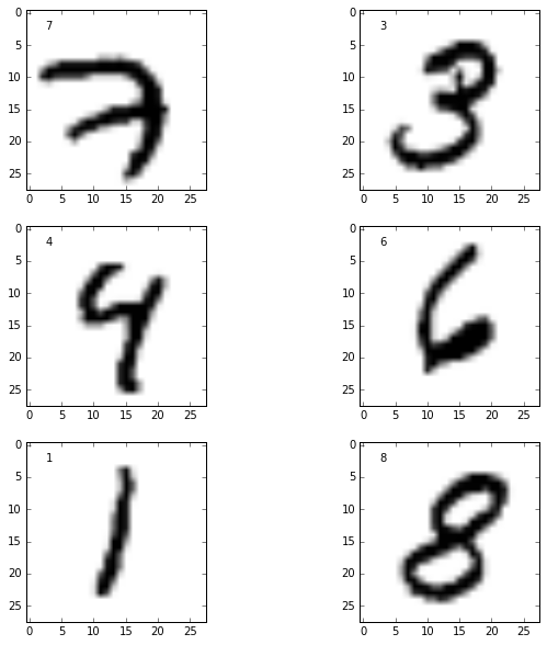
We have a training, validation and test set containing the images and labels. The images are flattened vectors of the 28x28 pixels, into 784 elements, and are stored as numpy arrays. The labels are “one-hot” vectors, the nth digit is represented as a vector which is 1 in the nth element, and zero everywhere else, also stored as numpy arrays.
Let’s peek at the actual data
import matplotlib.pyplot as plt
%matplotlib inline

left= 2.5
top = 2.5

fig = plt.figure(figsize=(10,10))

for i in range(6):
    ax = fig.add_subplot(3,2,i+1)
    im = np.reshape(mnist.train.images[i,:], [28,28])

    label = np.argmax(mnist.train.labels[i,:])
    ax.imshow(im, cmap='Greys')
    ax.text(left, top, str(label))
Next step: how to train a model
This problem is many-class classification, so we are going to train a model for each class. Specifically, we are going to train a set of weights that will be used to calculate a weighted sum of all the pixel intensities in the image. This weighted sum will be maximised when the weight model for the class matches the actual true class of the written digit. I.e. if the true label of the written digit is “3” then we want the weights corresponding to the class “3” to produce the largest weighted sum for that image.
The “evidence” for class is:
where the sum is over all the pixels of the image . are the weights for class in each pixel . is a bias that deals with class inbalances (e.g. maybe there are an overwhelming number of “3”’s in the data set compared to anything else so the “evidence” should favor “3” before any input data is even seen).
We need to turn this into a probability distribution: for any image the sum of “evidence” per class must equal 1. The probability distribution is defined using the softmax function (chosen so that it quickly becomes large for larger values):
where is the total number of classes.
Now implement in TensorFlow! Note all code below is taken from the tutorial, but the explainations are my own!
### THE SET UP

# A placeholder for the data (inputs and outputs)
# This represents any number (indicated by None)
# of the 784 pixel flattened images
x = tf.placeholder(tf.float32, [None, 784])
# This represents any number (indicated by None)
# of the 10 class "one-hot" vector of labels
y_ = tf.placeholder(tf.float32, [None, 10])


# The parameters of our model (to be learned): initialised to zero to start

# the weights for each pixel for each class
W = tf.Variable(tf.zeros([784, 10]))
# and the bias of each class
b = tf.Variable(tf.zeros([10]))


# The model!
y = tf.nn.softmax(tf.matmul(x, W) + b)


# A measure of the model precision using "cross-entropy"
cross_entropy = -tf.reduce_sum(y_*tf.log(y))


# The training step is minimising the cross_entropy via gradient descent
# with 0.01 as the learning rate
train_step = tf.train.GradientDescentOptimizer(0.01).minimize(cross_entropy)


# Initialise all the variable we have created
init = tf.initialize_all_variables()


### THE EXECUTION
sess = tf.Session()
sess.run(init)

# Do 1000 steps
for i in range(1000):

    # get random 100 data samples from the training set
    batch_xs, batch_ys = mnist.train.next_batch(100)

    # feed them to the model in place of the placeholders defined above
    sess.run(train_step, feed_dict={x: batch_xs, y_: batch_ys})
So the “stochastic” bit in the above was when we just grabbed 100 random data samples to iteratively train the model with in each step.
Evaluation with TensorFlow
# tf.argmax gives you the index of the highest entry in a tensor along some axis
# therefore checking if these indices are equal will return a boolean array
correct_prediction = tf.equal(tf.argmax(y,1), tf.argmax(y_,1))

# this accuracy is returning the mean value of an array of 1's and 0's
accuracy = tf.reduce_mean(tf.cast(correct_prediction, tf.float32))

# the following returns the accuracy on the TEST data, according to how
# accuracy and correct_prediction are defined above
print(sess.run(accuracy, feed_dict={x: mnist.test.images, y_: mnist.test.labels}))
0.9169
So our model is nearly 92% accurate, which is actually quite bad apparently!
How to get the data back!
From the docs:
A Tensor is a symbolic handle to one of the outputs of an Operation. It does
not hold the values of that operation’s output, but instead provides a means of
computing those values in a
TensorFlow.
So how do we look at the data we’ve created!
More from the docs:
After the graph has been launched in a session, the value of the Tensor can be
computed by passing it to Session.run()
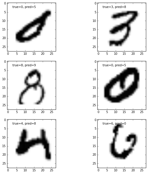
We get it returned from the graph node itself, “feeding” in the data we want used in the operation. See the example below that plots some of the classification failures.
correct_vals = sess.run(correct_prediction,
                        feed_dict={x: mnist.train.images, y_: mnist.train.labels})
pred_vals = sess.run(y, feed_dict={x: mnist.train.images} )

cntFalse = 0
for cv in correct_vals:
    if cv==False:
        cntFalse+=1
print cntFalse, "incorrect labels out of",  len(correct_vals)


fig = plt.figure(figsize=(10,10))

cntFalse = 0
for i, cv in enumerate(correct_vals):

    if cv==False:
        cntFalse +=1

        ax = fig.add_subplot(3,2,cntFalse)
        im = np.reshape(mnist.train.images[i,:], [28,28])

        label = np.argmax(mnist.train.labels[i,:])
        pred_label = np.argmax(pred_vals[i,:])

        ax.imshow(im, cmap='Greys')
        ax.text(left, top, 'true=' + str(label) + ', pred=' + str(pred_label))

    if cntFalse==6:
        break
4478 incorrect labels out of 55000

A visual inspection gives an idea of why this model is such a “failure” with only 92% accuracy.
It’s easy to see how the prediction could have occured in many cases: the predicted number often looks like it might share many high intensity pixels with the true number.
The model didn’t account explicitly for correlations between pixel intensities, e.g. if pixel is high intensity it’s very likely pixel will be too. I would imagine adding this kind of non-linearity to the model would easily bring the accuracy up to 97%+.