Linear regression (with multiple features)

Linear regression can be used when you want to predict single values rather than a class or category, and when a linear relationship between the features of the model and the value to predict is reasonably valid. The below follows closely the linear regression lecture from Andrew Ng’s Machine Learning course on Coursera.

Hypothesis in linear regression

From Andrew Ng’s ML course:

$h_\theta(x) = \theta_0x_0 + \theta_1 x_1 + … \theta_n x_n$

where $x_i$ is each feature in the model, and $x_0=1$ with $n$ the number of features. $\theta_i$ I refer to as the “feature parameters”.

Can re-write this in vector notation as

$h_\theta(x) = \Theta^Tx$

where $\Theta = [\theta_0, \theta_1, …, \theta_n]$ and $x = [x_0, x_1, … , x_n]$

These vectors have dimension $n+1$ to include the constant term/intercept $x_0=1$.

Cost function

The regression is performed by finding the $\Theta$ that minimize this cost function (Where $m$ is the number of data points):

$ J(\Theta) = \frac{1}{2m} \sum_{i+1}^m (\Theta^Tx^i - y^i)^2 $

The cost function is minimized here via gradient descent

Repeat {

$\theta_j := \theta_j - \alpha \frac{\delta J(\Theta)}{\delta \theta_j} = \theta_j - \alpha \frac{1}{m} \sum_{i+1}^m (h_\theta(x^i) - y^i)x^i $

}

simultaneously updating every feature parameter $j$. The index $i$ refers to the individual data points.

Feature scaling

Imagine you want to predict life expectancy based upon e.g. a person’s annual salary and the number of children they have. The two features have very different scales: salary $0 to $1,000,000+, whereas number of children could be 0 to 10+.

Imagine the possible contours drawn by constant values of the cost function in that 2D space: because the salary feature takes a huge range of values compared to the children feature they will be elongated in the salary dimension. If this is the case, gradient descent will have trouble finding the minimum as it will oscillate around a lot on its way to the global minimum (a large step in $\delta$[number of children] is equivalent to a tiny step in $\delta$[salary]).

To solve this problem we should set the features onto a similar scale, e.g. divide by the maximum values of each feature. A good aim is to get every feature approximately into a $-1<=x_i<=1$ range, though it’s ok if they are not exactly in this range, but are at least within the same order of magnitude as it. Possible ways to normalise:

divide by maximum value of feature (good if min is zero)
mean normalisation: replace $x_i$ by $(x_i - \mu_i)$ and divide by range
mean normalisation: replace $x_i$ by $(x_i - \mu_i)$ and divide by $s_i$

where $\mu_i$ is the average value of the $x_i$ feature in the training set, and $s_i$ is the standard deviation of $x_i$.

Learning rate $\alpha$

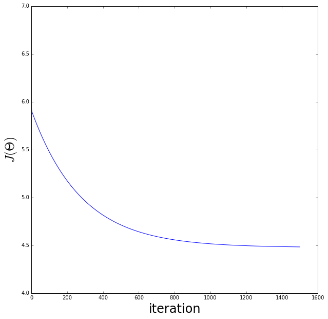
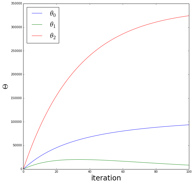
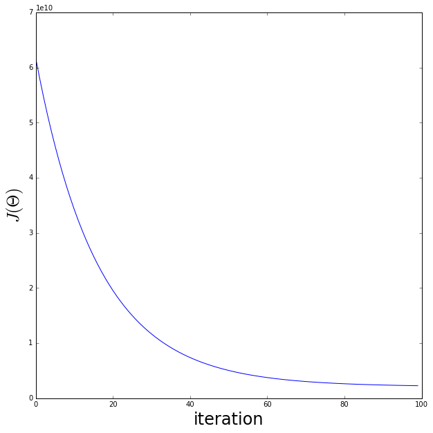
It is helpful to plot the value of $J(\Theta)$ as a function of the number of interations. If gradient descent is working properly $J(\Theta)$ should decrease after every iteration. When $J(\Theta)$ flattens off we can find the number of iterations it takes to converge (cost function no longer significantly decreases for new parameter updates). It is hard to tell in advance the number of iterations you will need for any particular application, but this can be played with.

Automatic convergence tests are often used to declare convergence, e.g. $\Delta J(\Theta)<10^{-3}$, but these should be checked afterwards by plotting $J(\Theta)$ for example.

If the gradient descent does not appear to be working, try using a smaller value for $\alpha$. But if $\alpha$ is too small gradient descent will be slow to converge, potentially prohibitively so.

Choosing features

Be careful when choosing features of the model. For example combining features together that are both very similarly related to what you are trying to predict could result in a better model.

Polynomial regression

It’s easy to see how we can extend this to polynomial regression by rewriting $h_\theta(x)$ e.g.

$h_\theta(x) = \theta_0 x_0 + \theta_1 x_1 + \theta_2 x_1^2 $

Warning: feature scaling becomes even more important here!

Normal equation method

Another method of solving for the minimum of the cost function, but this time analytically. This would replace gradient descent.

We can just differentiate the cost function with respect to each feature and set the differential to zero.

Normal equation:

Place all features into a matrix of $m$ rows (data points) by $n+1$ columns (features) called $X$. And also the values of the feature to be predicted into a $m$ rows (data points) by 1 vector called $y$ (because just single value to predict here):

$\Theta = (X^TX)^{-1}X^Ty $

Each training example gives a feature vector, and these are used to make the “design matrix” $X$. So each column feature vector $x$ is transposed and put into a row of $X$. The above equation gives the optimal value of $\Theta$ at the minimum of the cost value.

With this method feature scaling is not necessary. You also don’t need to choose a learning rate and don’t have to iterate.

However when there are are large number of features $n$ the Normal Equation is very slow if $n$ is large, because you have to invert $n$X$n$ matrix. The cost of inverting a matrix is $O(n^3)$ so should rethink using this if $n>10000$.

Python implementation of linear regression

In [18]:

import sklearn.linear_model as lm
import numpy as np
import matplotlib.pyplot as plt
%matplotlib inline


def h_theta(theta, X):
    """Take vector of feature parameters (theta) and matrix of features X  
       
       @param theta     size 1 x (n+1)
       @param X         size (n+1) x m (where feature x_0=1 for all data points)
       
       n = number of features
       m = number of data points
       
       Return the linear model hypothesis 
    """
    # check inner dimensions match
    if (theta.shape[1] != X.shape[0]):
        emsg = "dimension of feature vector and feature parameters are not equivalent: "
        emsg +="xi.shape = " + str(X.shape) + "theta.shape = " + str(theta.shape) + "\n"
        raise ValueError(emsg)
    
    return np.dot(theta, X)

    
def cost_function(theta, X, y):
    """Take vector of feature parameters (theta) and matrix of features (X), and vector of
       values to predict (y)
       
       @param theta     size 1 x (n+1)
       @param X         size (n+1) x m (where feature x_0=1 for all data points)
       @param y         size 1 x m (values to predict)
       
       n = number of features
       m = number of data points
       
       Return the cost function J
    """
    if (theta.shape[1] != X.shape[0]):
        emsg = "dimension of feature vector and feature parameters are not equivalent: "
        emsg +="xi.shape = " + str(X.shape) + "theta.shape = " + str(theta.shape) + "\n"
        raise ValueError(emsg)
        
    if np.max(y.shape) != X.shape[1]:
        emsg = "dimension of variables and feature parameters are not equivalent: "
        emsg +="xi.shape = " + str(X.shape) + "y.shape = " + str(y.shape) + "\n"
        raise ValueError(emsg)
      
    n = X.shape[0]  # number of features + 1
    m = X.shape[1]  # number of data points
    
    cf = 1./(2.*m)*np.dot( (h_theta(theta, X) - y),(h_theta(theta, X) - y).T )
    return cf[0,0]
    
    
def update_pars(theta, X, y, alpha):
    """Take vector of feature parameters (theta) and matrix of features (X), and vector of
       values to predict (y), and learning rate (alpha)
       
       @param theta     size 1 x (n+1)
       @param X         size (n+1) x m (where feature x_0=1 for all data points)
       @param y         size 1 x m (values to predict)
       @param alpha     learning rate of gradient descent
       
       n = number of features
       m = number of data points
       
       Return the updated parameters
    
    """

    if (theta.shape[1] != X.shape[0]):
        emsg = "dimension of feature vector and feature parameters are not equivalent: "
        emsg +="xi.shape = " + str(X.shape) + "theta.shape = " + str(theta.shape) + "\n"
        raise ValueError(emsg)
      
    n = X.shape[0]  # number of features + 1
    m = X.shape[1]  # number of data points

    return theta - alpha/float(m)*np.dot(h_theta(theta, X) - y, X.T)


def gradient_descent(theta, X, y, alpha, niter=100):
    """Take vector of feature parameters (theta) and matrix of features (X), and vector of
       values to predict (y), and learning rate (alpha)
       
       @param theta     size 1 x (n+1)
       @param X         size (n+1) x m (where feature x_0=1 for all data points)
       @param y         size 1 x m (values to predict)
       @param alpha     learning rate of gradient descent
       @param niter     number of iterations to do
       
       n = number of features
       m = number of data points
       
       Return the 
    
    """
    if (theta.shape[1] != X.shape[0]):
        emsg = "dimension of feature vector and feature parameters are not equivalent: "
        emsg +="xi.shape = " + str(X.shape) + "theta.shape = " + str(theta.shape) + "\n"
        raise ValueError(emsg)
      
    n = X.shape[0]  # number of features + 1
    m = X.shape[1]  # number of data points
    
    costs = []
    thetas = [theta]
    for i in range(niter):
        
        theta = update_pars(theta, X, y, alpha)
              
        thetas.append(theta)
        costs.append(cost_function(theta, X, y))
        
    return theta, costs, thetas

Test this implementation using the data sets supplied with exercise 1 of Andrew Ng’s course. The data below is simply the population of a city versus the profit of a food truck in that city.

In [19]:

# read in data
# The first column is the population of a city 
# The second column is the profit of a food truck in that city. 
# A negative value for profit indicates a loss.
data = np.genfromtxt('machine-learning-ex1/ex1/ex1data1.txt', delimiter=",")

# number of data points, number of features
m, n = data.shape
n -= 1
print "Data set has", n ,"feature(s) and", m , "data points"

x = data[:,0] 
y = data[:,1]

# Add x_0=1 term
ones = np.ones((1, m))
x = np.vstack((x, ones))
# first row is the actual feature values
# second row are the x_0=1


# Transpose y so matches x
y = np.reshape(y, (1,m))


# create initial feature vector, all zeros
theta = np.zeros((1, n+1))
print "On first iteration, value of cost function =", cost_function(theta, x, y)

Data set has 1 feature(s) and 97 data points
On first iteration, value of cost function = 32.0727338775

Visualize the cost function

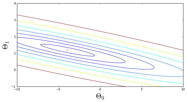
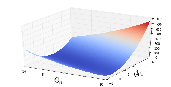
For a grid of likely $\Theta$ parameters calculate the values of the cost function and plot

In [20]:

# Grid over which we will calculate J
theta0_vals = np.linspace(-10, 10, 100) 
theta1_vals = np.linspace(-1, 4, 110)
THETA0, THETA1 = np.meshgrid(theta0_vals, theta1_vals)

# Calculate cost function values
Jvals = np.zeros((100,110))
for i in range(len(theta0_vals)):
    for j in range(len(theta1_vals)):
        t = np.reshape(np.asarray([theta1_vals[j], theta0_vals[i]]), (1, n+1))
        Jvals[i,j] = cost_function(t, x, y)

# find the minimum J value in the array
imin = np.unravel_index(Jvals.argmin(), Jvals.shape)
print "At minimum of array: Theta_0 =", theta0_vals[imin[0]], "Theta_1 =", theta1_vals[imin[1]]

# make a contour plot of an array Z. The level values are chosen automatically.
# contour(X,Y,Z)
# X and Y must both be 2-D with the same shape as Z, 
# or they must both be 1-D such that len(X) is the number of columns in Z 
# and len(Y) is the number of rows in Z.
        
# Plot Jvals as 20 contours spaced logarithmically between 0.01 and 100
fig = plt.figure(figsize=(10,5))
ax = fig.add_subplot(111)
ax.contour(theta0_vals, theta1_vals, Jvals.T, np.logspace(-2, 2, 20))
ax.plot(theta0_vals[imin[0]], theta1_vals[imin[1]], marker='x', color='red', linestyle='none')
ax.set_xlabel('$\Theta_0$', fontsize=24)
ax.set_ylabel('$\Theta_1$', fontsize=24)
#plt.axes().set_aspect('equal')
#ax.set_aspect('equal')

from mpl_toolkits.mplot3d import Axes3D
from matplotlib import cm
fig = plt.figure(figsize=(10,5))
ax = fig.gca(projection='3d')
ax.plot_surface(THETA0, THETA1, Jvals.T, rstride=1, cstride=1, cmap=cm.coolwarm,linewidth=0, antialiased=False)
ax.set_xlabel('$\Theta_0$', fontsize=24)
ax.set_ylabel('$\Theta_1$', fontsize=24)

At minimum of array: Theta_0 = -3.93939393939 Theta_1 = 1.20183486239

png

Do the regression

In [21]:

print "First check shapes of all inputs:"
print "Shape of feature matrix:", x.shape
print "Shape of values to predict:", y.shape
print "Shape of feature parameter vector:", theta.shape
print "Shape of resulting hypothesis:", h_theta(theta, x).shape, "\n"

niter = 1500
alpha = 0.01
final_theta, costs, all_thetas = gradient_descent(theta, x, y, alpha, niter)
print "Expectation: Theta_0 (intercept) =", theta0_vals[imin[0]], "Theta_1 (slope) =", theta1_vals[imin[1]]
print "Result: Theta_0 (intercept) =", final_theta[0,1], "Theta_1 (slope) =", final_theta[0,0]


theta0s = [t[0][0] for t in all_thetas ]
theta1s = [t[0][1] for t in all_thetas ]

fig = plt.figure(figsize=(10,10))
ax = fig.add_subplot(111)
ax.plot(theta0s, label='$ \\theta_0$')
ax.plot(theta1s, label='$ \\theta_1$')
ax.set_xlabel('iteration', fontsize=24)
ax.set_ylabel('$\Theta$', fontsize=24)
handles, labels = ax.get_legend_handles_labels()
ax.legend(prop={'size':24}, loc='upper left')

fig = plt.figure(figsize=(10,10))
ax = fig.add_subplot(111)
ax.plot(costs)
ax.set_xlabel('iteration', fontsize=24)
ax.set_ylabel('$J(\Theta)$', fontsize=24)

First check shapes of all inputs:
Shape of feature matrix: (2, 97)
Shape of values to predict: (1, 97)
Shape of feature parameter vector: (1, 2)
Shape of resulting hypothesis: (1, 97) 

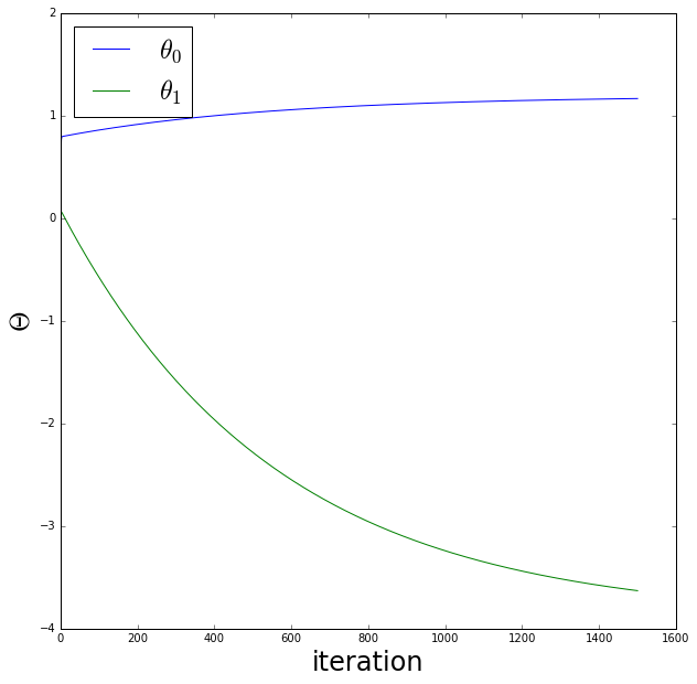
Expectation: Theta_0 (intercept) = -3.93939393939 Theta_1 (slope) = 1.20183486239
Result: Theta_0 (intercept) = -3.6302914394 Theta_1 (slope) = 1.16636235034

png

Plot the regression results

In [22]:

xpred = np.arange(0,25,0.1)
ypred = final_theta[0,1] + final_theta[0,0]*xpred


fig = plt.figure(figsize=(10,10))
ax = fig.add_subplot(111)
ax.plot(x[0,:], np.squeeze(y), color='red', marker='x', linestyle='none', label='training data')
ax.plot(xpred, ypred, color='black', linestyle='solid', label='linear regression')
ax.set_xlabel("Population of city (in 10,000's)", fontsize=24)
ax.set_ylabel("Profit of food truck (in $10,000's)", fontsize=24)
handles, labels = ax.get_legend_handles_labels()
ax.legend(prop={'size':12}, loc='upper left')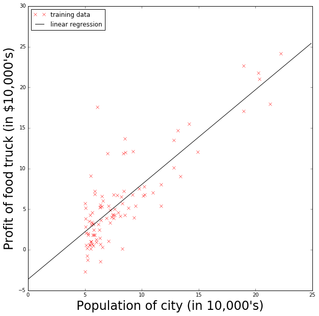

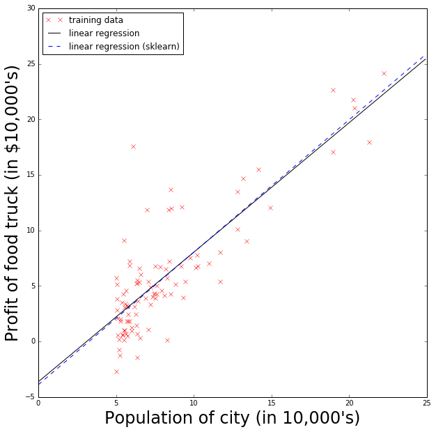
png

Compare to scikit-learn’s linear regression

In [23]:

linearReg = lm.LinearRegression(fit_intercept=True, normalize=False, copy_X=True, n_jobs=1)
linearReg.fit(x.T, y.T)

print "My result: Theta_0 (intercept) =", final_theta[0,1], "Theta_1 (slope) =", final_theta[0,0]
print "scikit learn result: Theta_0 (intercept) =", linearReg.intercept_[0], "Theta_1 (slope) =", linearReg.coef_[0][0]

ypred_sk = linearReg.intercept_[0] + linearReg.coef_[0][0]*xpred


fig = plt.figure(figsize=(10,10))
ax = fig.add_subplot(111)
ax.plot(x[0,:], np.squeeze(y), color='red', marker='x', linestyle='none', label='training data')
ax.plot(xpred, ypred, color='black', linestyle='solid', label='linear regression')
ax.plot(xpred, ypred_sk, color='blue', linestyle='dashed', label='linear regression (sklearn)')
ax.set_xlabel("Population of city (in 10,000's)", fontsize=24)
ax.set_ylabel("Profit of food truck (in $10,000's)", fontsize=24)
handles, labels = ax.get_legend_handles_labels()
ax.legend(prop={'size':12}, loc='upper left')

My result: Theta_0 (intercept) = -3.6302914394 Theta_1 (slope) = 1.16636235034
scikit learn result: Theta_0 (intercept) = -3.89578087831 Theta_1 (slope) = 1.19303364419

png

Now repeat with data that has multiple features

Again we test this using a data set supplied with exercise 1 of Andrew Ng’s course. The data below is a training set of housing prices in Portland, Oregon: the size of the house (in square feet), number of bedrooms, and the price of the house. Because house sizes are generally 1000’s of square feet and the number of bedrooms are < 10 we will need to use feature normalisation here.

In [24]:

# read in data
# A training set of housing prices in Portland, Oregon. 
# The first column is the size of the house (in square feet), 
# the second column is the number of bedrooms, 
# and the third column (to predict) is the price of the house.
data = np.genfromtxt('machine-learning-ex1/ex1/ex1data2.txt', delimiter=",")

# number of data points, number of features
m, n = data.shape
n -= 1
print "Data set has", n ,"features and", m , "data points"

x = data[:,:n] 
y = data[:,n]

# Add x_0=1 
ones = np.ones((m,1))
x = np.hstack((x, ones)).T

# Transpose y so matches x
y = np.reshape(y, (1,m))

# create initial feature vector
theta = np.ones((1, n+1))

Data set has 2 features and 47 data points

Plot the multivariate data

In [25]:

fig = plt.figure(figsize=(10,10))
ax = fig.add_subplot(111)
ax.plot(x[0,:], x[1,:], marker='.', linestyle='none')
ax.set_xlabel('size of house (sq. feet)', fontsize=24)
ax.set_ylabel('number of bedrooms', fontsize=24)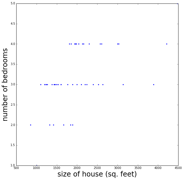

png

Feature normalization

The size of the house is on a much larger scale than the number of bedrooms

In [26]:

def feature_normalization(X):
    """Matrix of features X with size (nx1) by m where n is the number of features and 
       m is the number of data points. Return the normalized feature matrix Xnorm 
       where each feature has had its mean subtracted and has then been divided by its
       standard deviation (i.e. take mean of all data points along a row, std etc)
    """
    
    mus = np.mean(X, axis=1)
    stds = np.std(X, axis=1)

    Xnorm = (X.T-mus)/stds
    return Xnorm.T, mus, stds
    
xnorm = x.copy()
xnorm[:n,:], mus, stds = feature_normalization(x[:n,:])

In [27]:

print "Shape of feature matrix:", xnorm.shape
print "Shape of values to predict:", y.shape
print "Shape of feature parameter vector:", theta.shape
print "Shape of hypothesis:", h_theta(theta, xnorm).shape

alpha = 0.03
niter = 100
final_theta, costs, all_thetas = gradient_descent(theta, xnorm, y, alpha, niter)

theta0s = [t[0][0] for t in all_thetas ]
theta1s = [t[0][1] for t in all_thetas ]
theta2s = [t[0][2] for t in all_thetas ]

fig = plt.figure(figsize=(10,10))
ax = fig.add_subplot(111)
ax.plot(theta0s, label='$ \\theta_0$')
ax.plot(theta1s, label='$ \\theta_1$')
ax.plot(theta2s, label='$ \\theta_2$')
ax.set_xlabel('iteration', fontsize=24)
ax.set_ylabel('$\Theta$', fontsize=24)
handles, labels = ax.get_legend_handles_labels()
ax.legend(prop={'size':24}, loc='upper left')

fig = plt.figure(figsize=(10,10))
ax = fig.add_subplot(111)
ax.plot(costs)
ax.set_xlabel('iteration', fontsize=24)
ax.set_ylabel('$J(\Theta)$', fontsize=24)

Shape of feature matrix: (3, 47)
Shape of values to predict: (1, 47)
Shape of feature parameter vector: (1, 3)
Shape of hypothesis: (1, 47)

png

In [28]:

size = xnorm[0,:]
nbeds = xnorm[1,:]
ypred = final_theta[0,0]*size + final_theta[0,1]*nbeds + final_theta[0,2]*xnorm[2,:]

isort = np.argsort(size)


fig = plt.figure(figsize=(20,10))
ax = fig.add_subplot(121)
ax.plot(size[isort]*stds[0]+mus[0], np.squeeze(y[0, isort]), marker='.', linestyle='none')
ax.plot(size[isort]*stds[0]+mus[0], ypred[isort], color='red', linestyle='solid')
ax.set_xlabel('size of house (sq. feet)', fontsize=24)
ax.set_ylabel('House price', fontsize=24)

ax = fig.add_subplot(122)
ax.plot(xnorm[1,:]*stds[1]+mus[1], np.squeeze(y), marker='.', linestyle='none')
ax.plot(xnorm[1,:]*stds[1]+mus[1], ypred, color='red', marker='o', linestyle='none')
ax.set_xlabel('number of bedrooms', fontsize=24)
ax.set_ylabel('House price', fontsize=24)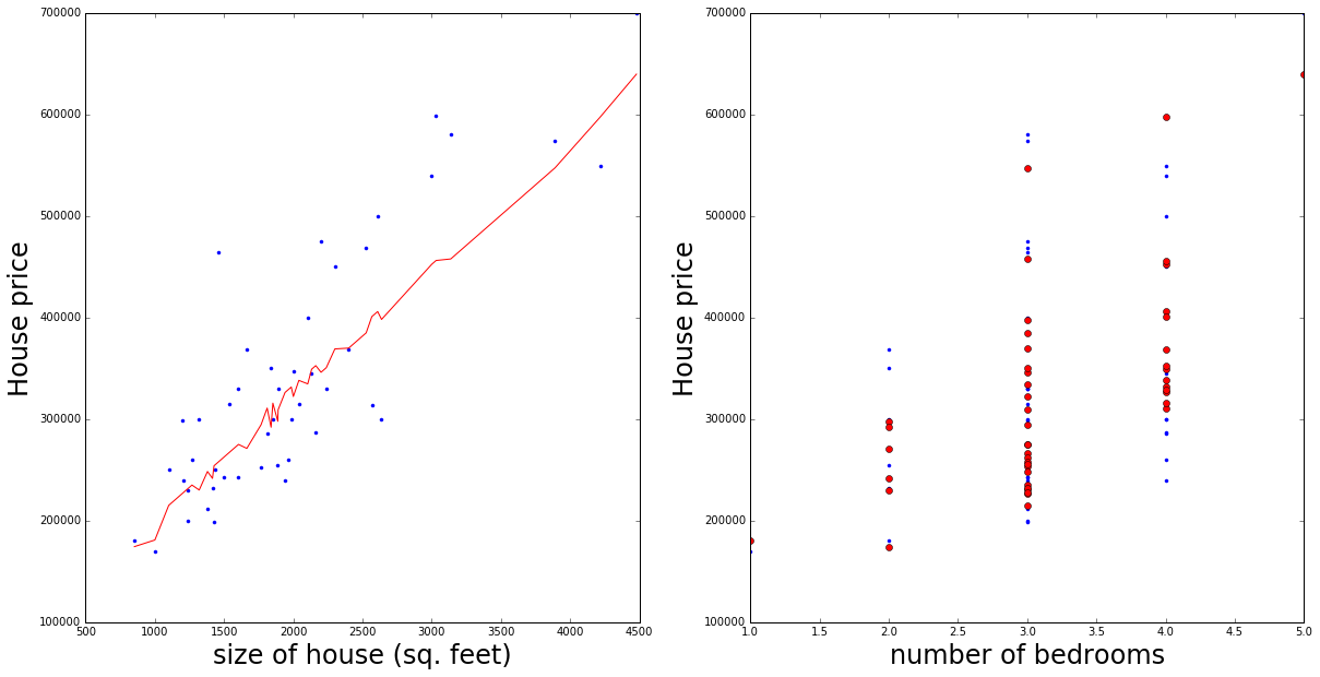

png

Compare to scikit-learn

In [29]:

linearReg = lm.LinearRegression(fit_intercept=True, normalize=True, copy_X=True, n_jobs=1)
linearReg.fit(x.T, y.T)

print "My result: Theta_0 (intercept) =", final_theta[0,2], "Theta_1 =", final_theta[0,1],
print "Theta_2 =", final_theta[0,0]
print "scikit learn result: Theta_0 (intercept) =", linearReg.intercept_[0], 
print "Theta_1 =", linearReg.coef_[0][0], "Theta_2 =", linearReg.coef_[0][1]

size_un = x[0,:]
nbeds_un = x[1,:]
ypred_sk = linearReg.coef_[0][0]*size_un + linearReg.coef_[0][1]*nbeds_un + linearReg.intercept_[0]

isort_sk = np.argsort(size_un)

fig = plt.figure(figsize=(20,10))
ax = fig.add_subplot(121)
ax.plot(size[isort]*stds[0]+mus[0], np.squeeze(y[0, isort]), marker='.', linestyle='none', label='data')
ax.plot(size[isort]*stds[0]+mus[0], ypred[isort], color='red', linestyle='solid', label='my linear regression')
ax.plot(size_un[isort_sk], ypred_sk[isort_sk], color='blue', linestyle='dashed', label='linear regression (sklearn)')
handles, labels = ax.get_legend_handles_labels()
ax.legend(prop={'size':12}, loc='upper left')
ax.set_xlabel('size of house (sq. feet)', fontsize=24)
ax.set_ylabel('House price', fontsize=24)

ax = fig.add_subplot(122)
ax.plot(nbeds*stds[1]+mus[1], np.squeeze(y[0, isort]), marker='.', linestyle='none', label='data')
ax.plot(nbeds*stds[1]+mus[1], ypred[isort], marker='o', color='red', linestyle='none', label='my linear regression')
ax.plot(nbeds_un[isort_sk], ypred_sk[isort_sk], marker='x', color='black', linestyle='none', label='linear regression (sklearn)')
handles, labels = ax.get_legend_handles_labels()
ax.legend(prop={'size':12}, loc='upper left')
ax.set_xlabel('size of house (sq. feet)', fontsize=24)
ax.set_ylabel('House price', fontsize=24)

My result: Theta_0 (intercept) = 324225.231435 Theta_1 = 8355.55697247 Theta_2 = 93661.3223261
scikit learn result: Theta_0 (intercept) = 89597.9095428 Theta_1 = 139.210674018 Theta_2 = -8738.01911233

png

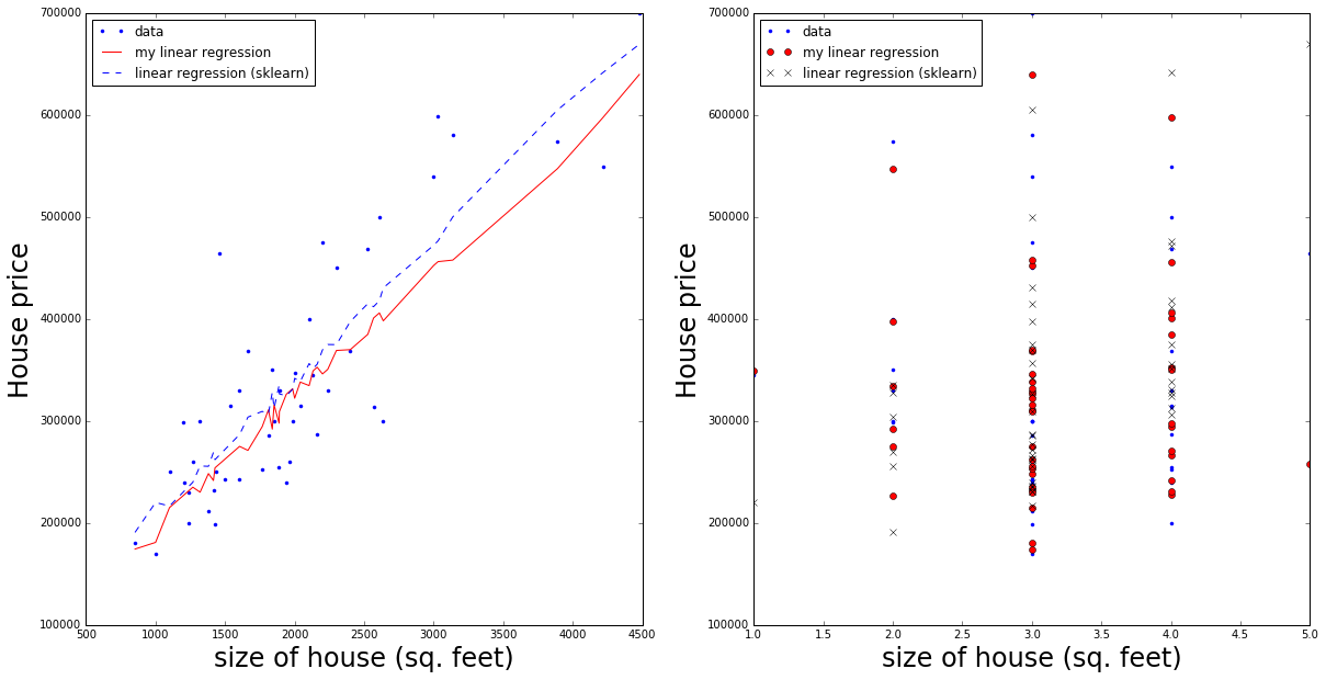
Obviously scikit-learn returns the feature parameters already un-normalised

Linear Regression