Logistic Regression for classification

This is similar to linear regression, except now the variable we want to predict can only take discrete values. E.g. this binary classification problem:

$ y \in {0, 1} $

0: negative class (e.g. absense of something, tumor is benign)
1: positive class (e.g. presense of something, tumor is malignant)

Therefore the logistic regression algorithm must always return a value for the hypothesis that is between 0 and 1.

Hypothesis in logistic regression

Again following Andrew Ng’s ML course, we want $0 \le h_\theta(x) \le 1$, so now:

$h_\theta(x) = g(\Theta^Tx)$

where $g(z) =\frac{1}{1+e^{-z}}$ and $g(z)$ is called the sigmoid function or logistic function. So:

$h_\theta(x) = \frac{1}{1+e^{-\Theta^Tx}}$

Let’s plot the sigmoid function below

In [123]:

import numpy as np
import matplotlib.pyplot as plt
%matplotlib inline

def sigmoid(z):
    """Return the value of the sigmoid function at z
    """
    return 1./(1+np.exp(-z))

z = np.arange(-20, 20, 1)
g = sigmoid(z)

fig = plt.figure(figsize=(10,10))
ax = fig.add_subplot(111)
ax.plot(z,g)
ymin = -0.1
ymax = 1.1
ax.plot([0,0],[ymin,ymax], color='black', linestyle='dotted')
ax.plot(z, np.ones(g.shape)*0.5, color='black', linestyle='dotted')
ax.set_ylim([ymin, ymax])
ax.set_xlabel('$z$', fontsize=24)
ax.set_ylabel('$g(z)$', fontsize=24)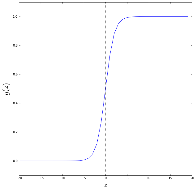

png

Note that $g(z)\ge 0.5$ when $z \ge 0$ so the hypothesis:

$h_\theta(x) = g(\Theta^Tx) \ge 0.5$ means $ \Theta^Tx \ge 0 $

and vice versa

$h_\theta(x) = g(\Theta^Tx) \le 0.5$ means $ \Theta^Tx \le 0 $

$h_\theta(x)$ is always bounded between 0 and 1.

Interpretation of hypothesis output

$h_\theta(x)$ is the probability that $y=1$ given input $x$ for a model parameterised by $\theta$, or:

$h_\theta(x) = p(y=1\mid x; \theta) $

So if the variable $x$ represented tumor size, and the hypothesis returned the value $h_\theta(x)=0.7$, there is a 70% probability that the tumor is malignant.

The code below shows a function defining the hypothesis for logistic regression.

In [124]:

def h_theta(theta, X):
    """Take vector of feature parameters (theta) and matrix of features X  
       
       @param theta     size 1 x (n+1)
       @param X         size (n+1) x m (where feature x_0=1 for all data points)
       
       n = number of features
       m = number of data points
       
       Return the logistic hypothesis 
    """
    return sigmoid(np.dot(theta, X))

Data

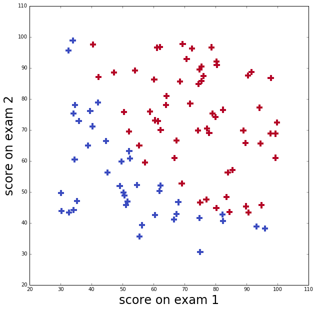
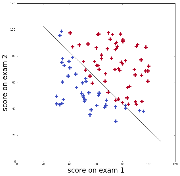
I’ll use data from Andrew Ng’s course to illustrate logistic regression in python. This data set is an applicant’s scores on two exams and the admissions decision.

The applicant was admitted if their scores were one of those in the upper right points (in red), and was not admitted if their scores were one in the lower left points (in blue)

In [125]:

data = np.genfromtxt('machine-learning-ex2/ex2/ex2data1.txt', delimiter=",")

# number of data points, number of features
m, n = data.shape
n -= 1
print "Data set has", n ,"feature(s) and", m , "data points"

fig = plt.figure(figsize=(10,10))
ax = fig.add_subplot(111)
ax.scatter(data[:,0], data[:,1], marker='+', s=150, linewidths=4, c=data[:,2], cmap=plt.cm.coolwarm)
ax.set_xlabel('score on exam 1', fontsize=24)
ax.set_ylabel('score on exam 2', fontsize=24)

Data set has 2 feature(s) and 100 data points

png

Cost function

We can’t simply plug in our logistic regression hypothesis into the same cost function we used for linear regression. This is because the sigmoid function is highly non linear and would result in a non-convex cost function that is not guaranteed to converge to the global minimum.

We need a cost function that would produce a “bowl shape” (a convex function) as a function of the parameters $\theta$. Therefore gradient descent can definitely converge to the global minimum.

The cost function for logistic regression will be:

$\begin{equation*} \mbox{Cost}(h_\theta(x),y) = \begin{cases} -\log(h_\theta(x)) \quad \quad \mbox{if} \quad y=1\\ -\log(1-h_\theta(x)) \quad \mbox{if} \quad y=0\\ \end{cases} \end{equation*}$

Let’s plot what we expect this to look like as a function of $h_\theta$ for $y=1$ and $y=0$

In [126]:

# know that logistic h_theta will output value between zero and 1 
ht = np.arange(0,1,0.01)
costy1 = -np.log10(ht)
costy2 = -np.log10(1.-ht)

fig = plt.figure(figsize=(10,10))
ax = fig.add_subplot(111)
ax.plot(ht, costy1, linestyle='solid', label='$y=1$')
ax.plot(ht, costy2, linestyle='solid', label='$y=0$')
ax.set_xlabel('$h_{\\theta}(x)$', fontsize=24)
ax.set_ylabel('Cost', fontsize=24)
handles, labels = ax.get_legend_handles_labels()
ax.legend(prop={'size':24}, loc='upper right')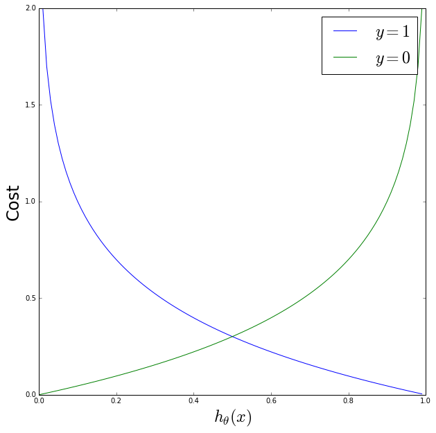

png

Focussing on the $y=1$ (blue) curve: the cost$=0$ when $h_\theta=1$, and as $h_\theta \rightarrow 0$ the cost $\rightarrow \infty$ which is the behavior we want. And the reverse is true for the $y=0$ (blue) curve.

Gradient descent

The update rule for the parameters $\theta$ in logistical regression looks identical to that of linear regression, but because the hypothesis has changed it is not exactly the same thing.

Repeat {

$\theta_j := \theta_j + \alpha \frac{\delta J(\Theta)}{\delta \theta_j} = \theta_j - \alpha \frac{1}{m} \sum_{i+1}^m (h_\theta(x^i) - y^i)x^i $

}

In [127]:

def cost_function(theta, X, y):
    """Take vector of feature parameters (theta) and matrix of features (X), and vector of
       values to predict (y)
       
       @param theta     size 1 x (n+1)
       @param X         size (n+1) x m (where feature x_0=1 for all data points)
       @param y         size 1 x m (values to predict)
       
       n = number of features
       m = number of data points
       
       Return the logistic cost function
    """
      
    n = X.shape[0]  # number of features + 1
    m = X.shape[1]  # number of data points
    
    
    cf = (1./float(m))*np.sum(-y*np.log(h_theta(theta, X)) - (1.-y)*np.log(1. - h_theta(theta, X)))
    
    return cf


def gradient(theta, X, y):
    """Calculate gradient of cost function
    """
    
    m = X.shape[1]  # number of data points
    return 1./float(m)*np.dot(h_theta(theta, X) - y, X.T)



x = data[:,:2]
y = data[:,2]

# Add x_0=1 term
ones = np.ones((1, m))
x = np.vstack((x.T, ones))

# first two rows are the actual feature values
# third row are the x_0=1


# Transpose y so matches x
y = np.reshape(y, (1,m))


# create initial feature vector, all zeros
theta = np.zeros((1, n+1))
print "On first iteration, value of cost function =", cost_function(theta, x, y)

On first iteration, value of cost function = 0.69314718056

Finding minimum of cost function

I’m going to use a built-in function from scipy instead of my own gradient descent (copying this stage of Ng’s course where he uses Matlab’s fminunc) though still using my functions for the cost function.

In [128]:

import scipy.optimize as op

Result = op.minimize(fun=cost_function, x0=theta, args=(x, y), method='TNC', jac=gradient)
optimal_theta = Result.x
print "Optimal theta =", optimal_theta
print "Cost function at minimum =", Result.fun

# Calculate the decision boundary line
plot_x1 = np.arange(20,110,1)
plot_x2 = -(optimal_theta[2] + optimal_theta[1]*plot_x1)/optimal_theta[0]


fig = plt.figure(figsize=(10,10))
ax = fig.add_subplot(111)
ax.plot(plot_x1, plot_x2, color='black', linestyle='solid', label='Decision boundary')
ax.scatter(data[:,0], data[:,1], marker='+', s=150, linewidths=4, c=data[:,2], cmap=plt.cm.coolwarm)
ax.set_xlabel('score on exam 1', fontsize=24)
ax.set_ylabel('score on exam 2', fontsize=24)

Optimal theta = [  0.20623159   0.20147149 -25.16131872]
Cost function at minimum = 0.203497701589

png

Predictions

To evaluate how well the statistical model does compare the predicted class to the actual class.

In [129]:

def predict(theta, X):
    """Take vector of feature parameters (theta) and matrix of features X and predict class
       (0 or 1)
       
       @param theta     size 1 x (n+1)
       @param X         size (n+1) x m (where feature x_0=1 for all data points)
       
       n = number of features
       m = number of data points
    
    """
    m = X.shape[1]
    p = np.zeros((m,1)) 
    p[np.where(h_theta(theta, X)>0.5)] = 1
    return p.T

def evaluate(y, p):
    """Evaluate percentage of correct classifications
    
       @param y    actual classifications 1xm
       @param p    predicted classifications 1xm
    """
    m = y.shape[1]

    return np.sum(y==p)/float(m)
    
p = predict(optimal_theta, x)
print evaluate(y,p)*100 ,"percent of classifications on the training data were correct"

89.0 percent of classifications on the training data were correct

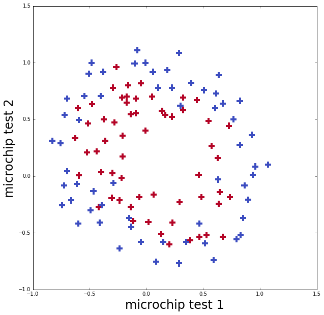
Non linear decision boundary

This data set (from Andrew Ng’s course) is the outcome of two different tests on microchips to determine if they are functioning correctly. As can be seen from the plot of the data, the boundary between functioning and not functioning is clearly not linear.

Applying logistic regression as we just did will not end up performing well on this dataset because it will only be able to find a linear decision boundary.

In [130]:

data = np.genfromtxt('machine-learning-ex2/ex2/ex2data2.txt', delimiter=",")

# number of data points, number of features
m, n = data.shape
n -= 1
print "Data set has", n ,"feature(s) and", m , "data points"


x = data[:,:2]
y = data[:,2]

# Add x_0=1 term
ones = np.ones((1, m))
x = np.vstack((x.T, ones))

# first two rows are the actual feature values
# third row are the x_0=1


# Transpose y so matches x
y = np.reshape(y, (1,m))

fig = plt.figure(figsize=(10,10))
ax = fig.add_subplot(111)
ax.scatter(data[:,0], data[:,1], marker='+', s=150, linewidths=4, c=data[:,2], cmap=plt.cm.coolwarm)
ax.set_xlabel('microchip test 1', fontsize=24)
ax.set_ylabel('microchip test 2', fontsize=24)

Data set has 2 feature(s) and 118 data points

png

Therefore we shall follow the exercise in Ng’s course and re-map the two features onto new features which are all the possible polynomial terms of $x_1$ and $x_2$ up to a degree of 6.

A logistic regression classifier trained on this higher-dimension feature vector will have a more complex decision boundary and will appear nonlinear when drawn in the 2-D plot.

In [131]:

def sum_nums(n):
    """Sum up numbers from 1 to n+1"""
    
    if n==0:
        return 1
    else:
        return sum_nums(n-1) + n+1

def map_to_poly(x1, x2, degree=6):
    """Map two features into nth degree polynomial space
    """
    if isinstance(x1, np.ndarray):
        m = len(x1)
    else:
        m=1
    n = sum_nums(degree)
    xpoly = np.ones((n,m))
    # the bottom row will be the x_0=1 feature
    
    ifeat = n-2
    for i in range(1, degree+1):
        for j in range(0, i+1):
            feat = pow(x1,i-j)*pow(x2,j)  # mx1
            xpoly[ifeat,:] = feat
            ifeat -= 1

    return xpoly


X = map_to_poly(x[0,:], x[1,:])
n = X.shape[0]
print "There are now", n ,"features"

There are now 28 features

Regularised cost function

Because of the high order terms being used in the $x_1$, $x_2$ to $y$ relationship we will need to avoid overfitting by using regularisation.

In [132]:

def reg_cost_function(theta, X, y, lam):
    """Take vector of feature parameters (theta) and matrix of features (X), and vector of
       values to predict (y)
       
       @param theta     size 1 x (n+1)
       @param X         size (n+1) x m (where feature x_0=1 for all data points)
       @param y         size 1 x m (values to predict)
       @param lam       lambda parameter
       
       n = number of features
       m = number of data points
       
       Return the regularised logistic cost function
    """
      
    n = X.shape[0]  # number of features + 1
    m = X.shape[1]  # number of data points
    
    
    cf = (1./float(m))*np.sum(-y*np.log(h_theta(theta, X)) - (1.-y)*np.log(1. - h_theta(theta, X)))
    
    # add regularised term
    cf += lam/(2.*m)*np.sum(theta[:-1])
    
    return cf


def reg_gradient(theta, X, y, lam):
    """Calculate gradient of the regularised cost function
    
       @param theta     size 1 x (n+1)
       @param X         size (n+1) x m (where feature x_0=1 for all data points)
       @param y         size 1 x m (values to predict)
       @param lam       lambda parameter
       
       return vector of gradient of cost function
    """

    
    m = X.shape[1]  # number of data points
    dcost = 1./float(m)*np.dot(h_theta(theta, X) - y, X.T)

    # regularise
    dcost[0,:-1] += theta[:-1]*(lam/float(m))
    
    return dcost


# create initial feature vector, all zeros
theta = np.zeros((1, n))
lam = 1
print "On first iteration, value of cost function =", reg_cost_function(theta, X, y, lam)

On first iteration, value of cost function = 0.69314718056

In [133]:

Result = op.minimize(fun=reg_cost_function, x0=theta, args=(X, y, lam), 
                     method='TNC', jac=reg_gradient)

optimal_theta = Result.x
print "Optimal theta =", optimal_theta
print "Cost function at minimum =", Result.fun

Optimal theta = [-0.93550801 -0.13804201 -0.32917181  0.00961561 -0.29638538  0.0208285
 -1.04396483 -0.46790766 -0.29276903 -0.27804401 -0.05490412 -0.20901429
 -0.23663768 -1.20129274 -0.27174423 -0.619998   -0.06288687 -1.46506516
 -0.18067778 -0.36458165 -0.36770494  0.12444377 -1.41319176 -0.91708231
 -2.02173833  1.18590364  0.62478646  1.27422034]
Cost function at minimum = 0.414779521282

In [135]:

def plotDecisionBoundary(theta, X, y, ax):
    """Plots the data points X and y into a new figure with the 
       decision boundary defined by theta

       Plots the data points colored blue for the positive examples 
       and red for the negative examples. X is assumed to be either:
       
       1) 3xM matrix, where the last row is an all-ones column for the 
          intercept.
       2) NxM, N>3 matrix, where the last row is all-ones
    """

    # Plot Data
    ax.scatter(X[-2,:], X[-3,:], marker='+', s=150, linewidths=4, 
           c=y, cmap=plt.cm.coolwarm, label="data")
    
    if X.shape[0] <= 3:
        # Only need 2 points to define a line, so choose two endpoints
        plot_x = [np.min(X[-2,:])-2,  np.max(X[-2,:])+2]

        # Calculate the decision boundary line
        plot_y = (-1./theta[0])*(theta[1]*plot_x + theta[2])

        # Plot, and adjust axes for better viewing
        ax.plot(plot_x, plot_y, label="decision boundary")
    
        ax.set_xlim([30, 100])
        ax.set_ylim([30, 100])
                  
    else:
        # Here is the grid range
        u = np.linspace(-1, 1.5, 50)
        v = np.linspace(-1, 1.5, 50)

        z = np.zeros((len(u), len(v)))
        
        # Evaluate z = theta*x over the grid
        for i in range(len(u)):
            for j in range(len(v)):
                z[i,j] = np.dot(map_to_poly(u[i], v[j]).T,theta.T)

        z = z.T # important to transpose z before calling contour

        # Plot z = 0
        # Notice you need to specify the range [0, 0]
        ax.contour(u, v, z, [0,0.001], linewidth=2, color='black')


fig = plt.figure(figsize=(10,10))
ax = fig.add_subplot(111)
plotDecisionBoundary(optimal_theta, X, y, ax)
ax.set_xlabel('microchip test 1', fontsize=24)
ax.set_ylabel('microchip test 2', fontsize=24)
ax.set_title('With regularisation parameter $\lambda=1$', fontsize=24)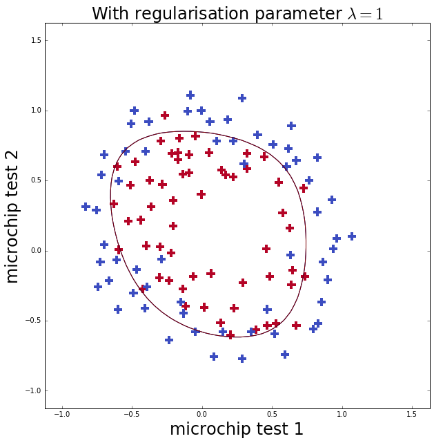

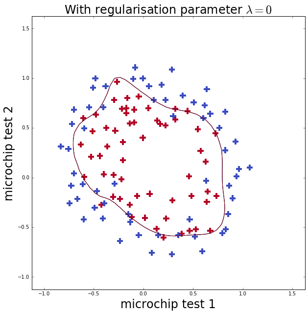
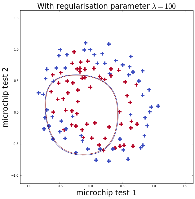
png

Over-fitting and under-fitting

Now I repeat the fit with less ($\lambda=0$, well none) and more ($\lambda=100$) regularlisation. The first case should cause over-fitting, which you can see as it gets more training classifications correct than $\lambda=1$ but the boundary is more complicated. The second case should cause under-fitting, where below you can see that the model does not fit the training data well at all.

In [136]:

lam = 0
overfit_Result = op.minimize(fun=reg_cost_function, x0=theta, args=(X, y, lam), 
                     method='TNC', jac=reg_gradient)

overfit_theta = overfit_Result.x

lam = 100
underfit_Result = op.minimize(fun=reg_cost_function, x0=theta, args=(X, y, lam), 
                     method='TNC', jac=reg_gradient)

underfit_theta = underfit_Result.x


fig = plt.figure(figsize=(10,10))
ax = fig.add_subplot(111)
plotDecisionBoundary(overfit_theta, X, y, ax)
ax.set_xlabel('microchip test 1', fontsize=24)
ax.set_ylabel('microchip test 2', fontsize=24)
ax.set_title('With regularisation parameter $\lambda=0$', fontsize=24)


fig = plt.figure(figsize=(10,10))
ax = fig.add_subplot(111)
plotDecisionBoundary(underfit_theta, X, y, ax)
ax.set_xlabel('microchip test 1', fontsize=24)
ax.set_ylabel('microchip test 2', fontsize=24)
ax.set_title('With regularisation parameter $\lambda=100$', fontsize=24)

png