Generating galaxies using PCA and Gaussian Process

Galaxies have a wide range of colors depending on the kinds of stars that make them up, the ages of those stars, and properties of dust in the interstellar space. And probably a bunch of other stuff too. However although there is technically an infinite possible number of galaxy spectra, there are not limitless possibilities since the distribution of emitted flux with wavelength depends upon a set of well-defined physical processes determined by star formation and atomic physics.

Given some galaxy color (ratio of its flux at adjacent wavelengths), we want to simulate its probable underlying galaxy spectrum, and one that is drawn from a continuous distribution. We need some way of defining this distribution such that it can produce any possible galaxy spectrum, but never an unphysical galaxy spectrum (i.e. one that cannot be produced by radiation from stars+dust).

We have an idea of what the range of galaxy spectra in the universe are like so we start from a set of discrete galaxy spectra we think (assume) roughly span the real range of galaxy spectra.

Plotted below is the set of discrete galaxy spectra I will use.

In [23]:

from sklearn.decomposition import PCA as sklPCA
import matplotlib.pyplot as plt
%matplotlib inline
import numpy as np
import sedFilter
import photometry as phot
import sedMapper


### Read the spectra into a python dictionary
listOfSpectra = 'brown_masked.seds'                             
pathToSpectra = '/mnt/drive2/repos/PhotoZDC1/sed_data/'
sedDict = sedFilter.createSedDict(listOfSpectra, pathToSpectra)
nSpectra = len(sedDict)
print "Number of spectra =", nSpectra

### Plot all together
fig = plt.figure(figsize=(10,10))
ax = fig.add_subplot(111)
sedFilter.plotSedFilter(sedDict, ax)

Adding SED Arp_118_spec to dictionary
Adding SED Arp_256_N_spec to dictionary
Adding SED Arp_256_S_spec to dictionary
Adding SED CGCG_049-057_spec to dictionary
.....
Adding SED UGCA_219_spec to dictionary
Adding SED UGCA_410_spec to dictionary
Adding SED UM_461_spec to dictionary
Number of spectra = 129

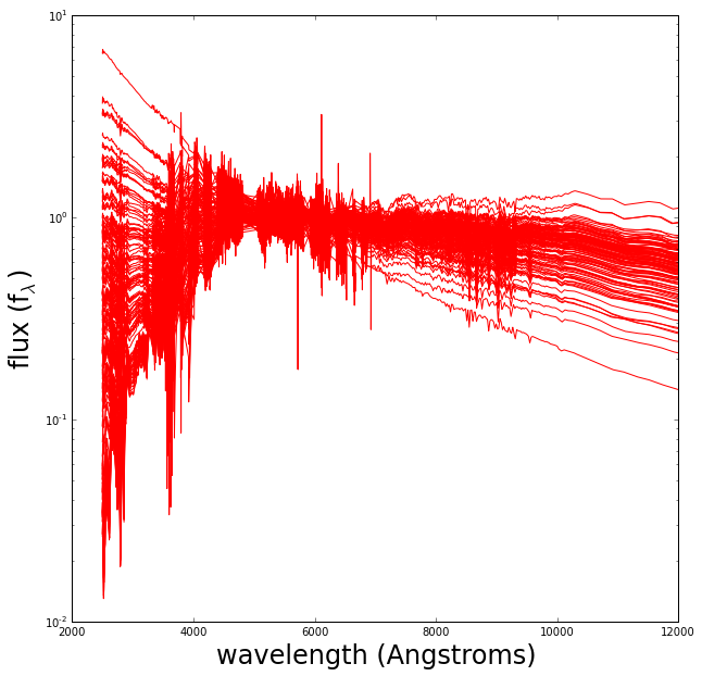
Each one of these discrete spectra has colors associated with it (color is the ratio of integrated flux within two neighboring wavelength regions). Given any “real” set of galaxy colors we want to produce a likely underlying spectrum.

The color is estimated from the flux within a series of filters that define the wavelength regions (for this case these are plotted below).

In [24]:

### Filter set to calculate colors
listOfFilters = 'LSST.filters'  
pathToFilters = '/mnt/drive2/repos/PhotoZDC1/filter_data/'
filterList = sedFilter.getFilterList(listOfFilters, pathToFilters)
filterDict = sedFilter.createFilterDict(listOfFilters, pathToFilters)
nFilters = len(filterList)
print "Number of filters =", nFilters


### Plot all together
fig = plt.figure(figsize=(10,10))
ax = fig.add_subplot(111)
sedFilter.plotSedFilter(filterDict, ax, isSED=False)

Adding filter LSST_u to dictionary
Adding filter LSST_g to dictionary
Adding filter LSST_r to dictionary
Adding filter LSST_i to dictionary
Adding filter LSST_z to dictionary
Adding filter LSST_y to dictionary
Number of filters = 6

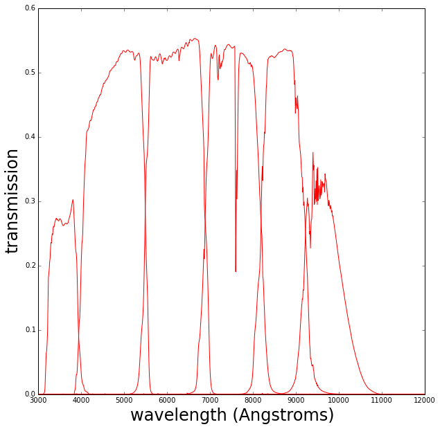
We want to define a relationship between the “observable”, the galaxy colors, and the spectrum we wish to predict.

It is a natural choice to decompose the spectra into a representative basis of “eigenspectra” using Principal Component Analysis (PCA). This is because in the simplest sense a galaxy spectrum is just a sum of different spectra of stars. The distribution of galaxy spectra could be then defined by the distribution of eigenvalue sets corresponding to the different eigenspectra, as derived from our set of discrete spectra.

We then need to make a mapping between color and a particular set of eigenvalues in order to reconstruct a galaxy spectrum given any set of galaxy colors. We don’t know what functional form this mapping relationship might take, and ideally we don’t want to restrict any model options, or be too flexible and allow for over-fitting that would render the derived mapping useless for any galaxies not within the original discrete set of spectra.

The Gaussian Process is a Bayesian method that assigns a set of prior probabilities to every possible function (e.g. higher probabilities to smooth functions, Occam’s razor) that could explain some observed data. The problem becomes tractable because you require estimates of the functional form only at particular points in the variable space (in this case galaxy colors). Once the prior probabilities for the set of functions are confronted with data points, their combination leads to a posterior distribution for the functions. It is the statistical properties of the resulting posterior distribution that supply the inference of the output (here eigenvalue set) given new input variables (here galaxy colors).

A covariance function used in the Gaussian Process decides the form the prior probabilities will take, by defining the shape of the prior probability distribution, and having a characteristic length scale to control quickly the prior probability changes over the function space. The covariance function is a function of the input variables. I think this is what makes the problem tractable, because the computation required is just the inversion of a matrix that is the size of the dimensionality of the data set.

The use of this method is not my idea and an original implementation can be found here.

In [25]:

### Wavelength grid to do PCA on
minWavelen = 2999.
maxWavelen = 12000.
nWavelen = 10000

                 
### Calculate all spectra colors, do PCA and train GP

ncomp = nSpectra  # keep all components for now

# pre-calculated colors for these spectra
color_file = "brown_colors_lsst.txt" 

# parameters for Gaussian Process covariance function
corr_type = 'cubic'
theta0 = 0.2


pcaGP = sedMapper.PcaGaussianProc(sedDict, filterDict, color_file, ncomp, 
                                  minWavelen, maxWavelen, nWavelen,
                                  corr_type, theta0)
colors = pcaGP._colors
spectra = pcaGP._spectra
waveLen = pcaGP._waveLen                # wavelength grid
meanSpectrum = pcaGP.meanSpec           # mean spectrum
eigenvalues = pcaGP.eigenvalue_coeffs # eigenvalues for each spectrum

Colors already computed, placing SEDs in array ...
On SED 1 of 129 NGC_4254_spec
On SED 2 of 129 NGC_6240_spec
On SED 3 of 129 UGC_06850_spec
.....
On SED 127 of 129 NGC_1144_spec
On SED 128 of 129 NGC_1068_spec
On SED 129 of 129 NGC_2623_spec
Mean spectrum shape: (10000,)
Eigenspectra shape: (129, 10000)
Eigenvalues shape: (129, 129)
Number of unique colors in SED set 129 total number of SEDs = 129

Plotting the first two eigenvalues shows that eigenvalue 1 gives a strong indication of galaxy color. A galaxy is “redder” if the “color” value is larger, and “bluer” if the value is smaller.

Very roughly a “blue” galaxy is star-forming and a “red” is old and no longer forming stars.

In [26]:

# plot distribution of first two eigenvalues
cm = plt.cm.get_cmap('hot')
fig = plt.figure(figsize=(10,10))
ax = fig.add_subplot(111)
cb = ax.scatter(eigenvalues[:,0], eigenvalues[:,1], c=colors[:,0], s=35, cmap=cm)
ax.set_xlabel('$e_1$', fontsize=24)
ax.set_ylabel('$e_2$', fontsize=24)
cbar = plt.colorbar(cb)
cbar.set_label('color', rotation=270, fontsize=24)
ax.set_xlim([-0.015, 0.005])
ax.set_ylim([-0.002, 0.004])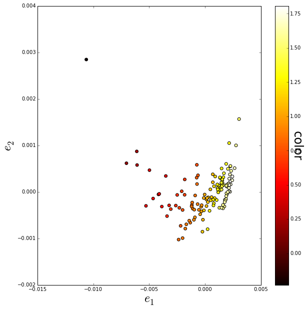

Now let’s do a test where we retrain the Gaussian process after removing one of the spectra, then try to see how well it reconstructs the missing spectrum.

In [27]:

### Leave out each SED in turn
delta_mag = np.zeros((nSpectra, nFilters))
performance = []
for i, (sedname, spec) in enumerate(sedDict.items()):
    
    print "\nOn SED", i+1 ,"of", nSpectra
    

    ### Retrain GP with SED removed
    nc = nSpectra-1
    pcaGP.reTrainGP(nc, i)
    
    
    ### Reconstruct SED
    sed_rec = pcaGP.generateSpectrum(colors[i,:])
        
    
    ### Calculate colors of reconstructed SED
    pcalcs = phot.PhotCalcs(sed_rec, filterDict)

    
    ### Get array version of SED back
    wl, spec_rec = sed_rec.getSedData(minWavelen, maxWavelen, nWavelen)
    
    
    ### Plot
    fig = plt.figure(figsize=(10,10))
    ax = fig.add_subplot(111)
    ax.plot(waveLen, spectra[i,:], color='blue', label='true')
    ax.plot(wl, spec_rec, color='red', linestyle='dashed', label='estimated')
    ax.plot(waveLen, meanSpectrum, color='black', linestyle='dotted', label='mean')
    ax.set_xlabel('wavelength (angstroms)', fontsize=24)
    ax.set_ylabel('flux', fontsize=24)
    handles, labels = ax.get_legend_handles_labels()
    ax.legend(loc='lower right', prop={'size':12})
    ax.set_title(sedname, fontsize=24) 
    y1, y2 = ax.get_ylim()
    typeg = 'red'
    if (colors[i,0]<0.5):
        typeg = 'blue'
    annotate  = "color = {0:.2f} ({1:s})\n".format(colors[i,0],typeg)
    ax.text(8000, 0.85*y2, annotate, fontsize=18, fontweight='bold')
    
    
    ### Break after 4
    if (i>3):
        break

On SED 1 of 129
Mean spectrum shape: (10000,)
Eigenspectra shape: (128, 10000)
Eigenvalues shape: (128, 128)
Number of unique colors in SED set 128 total number of SEDs = 128

On SED 2 of 129
Mean spectrum shape: (10000,)
Eigenspectra shape: (128, 10000)
Eigenvalues shape: (128, 128)
Number of unique colors in SED set 128 total number of SEDs = 128

On SED 3 of 129
Mean spectrum shape: (10000,)
Eigenspectra shape: (128, 10000)
Eigenvalues shape: (128, 128)
Number of unique colors in SED set 128 total number of SEDs = 128

On SED 4 of 129
Mean spectrum shape: (10000,)
Eigenspectra shape: (128, 10000)
Eigenvalues shape: (128, 128)
Number of unique colors in SED set 128 total number of SEDs = 128

On SED 5 of 129
Mean spectrum shape: (10000,)
Eigenspectra shape: (128, 10000)
Eigenvalues shape: (128, 128)
Number of unique colors in SED set 128 total number of SEDs = 128

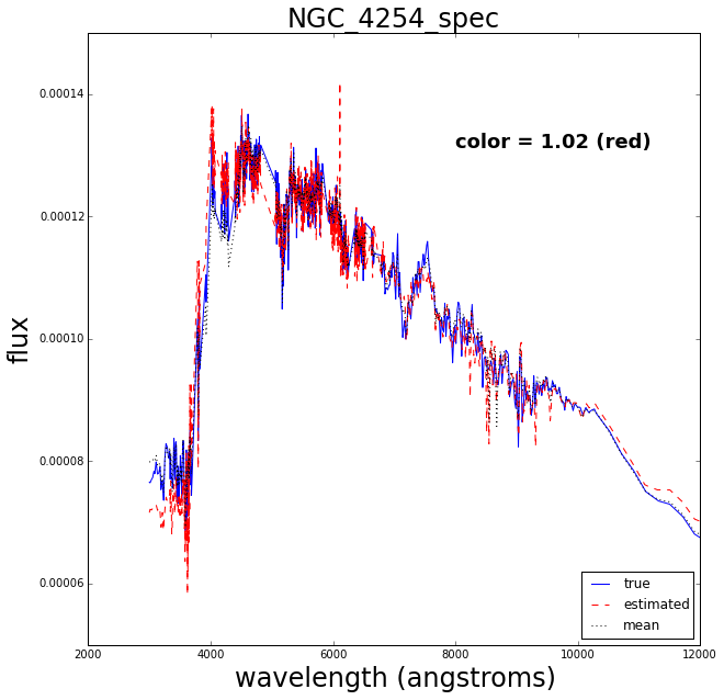
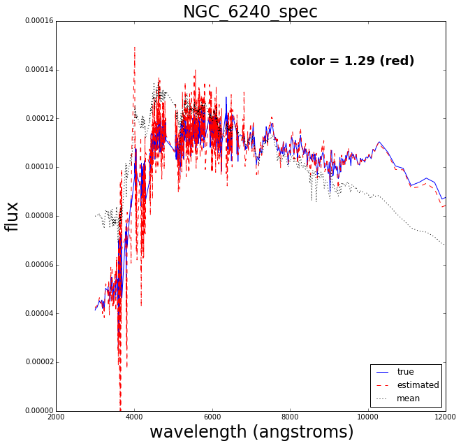
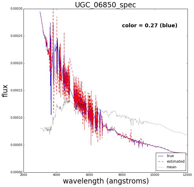
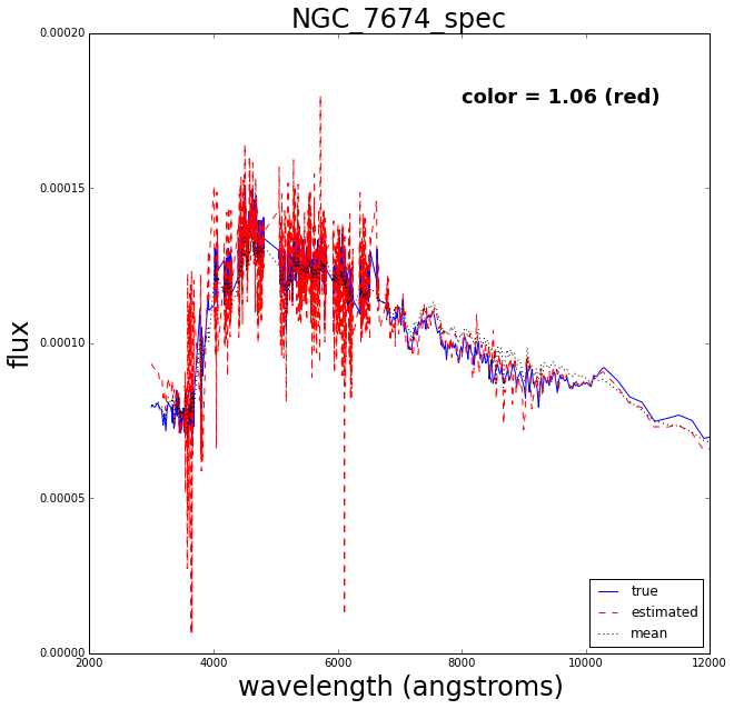
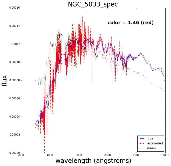
The blue solid line is the true spectrum, the dashed red is the reconstructed spectrum and the dotted mean is the mean over the 129 spectra.

The reconstruction works pretty well.