Information, noise and the atmosphere
Observing galaxies
To do extragalactic astronomy we need to measure a galaxy spectrum (a measure of the flux it emits at each wavelength) so we can find out what kind of galaxy it is and how far away it is. The structure of the spectrum, its overall shape and small scale details of its absorption and emission lines, tells us these properties.
Plotted below is an example of a galaxy spectrum.
In [45]:
import numpy as np
import matplotlib.pyplot as plt
%matplotlib inline

galaxy = np.loadtxt('NGC_4579_spec.dat')

fig = plt.figure(figsize=(5,5))
ax = fig.add_subplot(111)
ax.plot(galaxy[:,0], galaxy[:,1], color="black")
ax.set_xlim([0, 12000])
ax.set_xlabel('wavelength (angstroms)', fontsize=24)
ax.set_ylabel('flux', fontsize=24)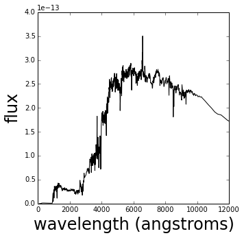
However it’s hard to measure a galaxy spectrum, obtaining enough signal at each wavelength takes potentially hours of observation time. This means that accumulating samples that contain millions of galaxies can take years, or more likely, decades. In fact some galaxies can’t be measured this way at all because they are just too faint.
Solution: measure the flux across a whole region of wavelengths instead of at individual wavelengths. This data is both faster to collect and still viable for very faint galaxies as there is more signal per data point.
Different filters are added in front of the telescope so only light of certain wavelengths can pass through. The plots below demonstrates this; they show a set of possible filters represented by their transmission functions, which are the probability of a photon of light making it through and being detected. Overplotted for illustration purposes is an example galaxy spectrum. All the flux from the galaxy that lies within the blue filter is added together (integrated) and so on for the other 5 filters plotted in different colors leaving (in this example) just 6 measurements of the galaxy’s flux.
The ideal filters (left hand side) show that all the light within the filter region is detected (as transmission probability=1 across the wavelength range of the filter, and is equal to 0 outside), but this is not what happens in practice.
In reality is not possible to fabricate such perfect filters, and the quality of the filters also degrades over time. In addition to this the detection probability is affected by the precision of the reflection by the telescope’s mirrors, the efficiency of the detector that measures the photons, and the transmission properties of light through the atmosphere. In short, the transmission of the filters is not constant from observation to observation.
And in reality, on average, we end up with something like the right hand side below.
In [46]:
filters = ['tophat_LSST_u.res', 'tophat_LSST_g.res', 'tophat_LSST_r.res',
           'tophat_LSST_i.res', 'tophat_LSST_z.res', 'tophat_LSST_y.res']

fig = plt.figure(figsize=(15,8))
ax = fig.add_subplot(121)
ax.plot(galaxy[:,0], galaxy[:,1]/np.max(galaxy[:,1]), color='black')

colors=['b','c','g','y','r','m']
for i,f in enumerate(filters):
    filt = np.loadtxt(f)
    ax.plot(filt[:,0], filt[:,1], color=colors[i], linewidth=2)

ax.set_xlim([0, 12000])
ax.set_ylim([0, 1.1])
ax.set_xlabel('wavelength (angstroms)', fontsize=24)
ax.set_ylabel('Transmission probability', fontsize=24)

filters = ['LSST_u.res', 'LSST_g.res', 'LSST_r.res',
           'LSST_i.res', 'LSST_z.res', 'LSST_y.res']

ax = fig.add_subplot(122)
ax.plot(galaxy[:,0], galaxy[:,1]/np.max(galaxy[:,1]), color='black')

colors=['b','c','g','y','r','m']
for i,f in enumerate(filters):
    filt = np.loadtxt(f)
    ax.plot(filt[:,0], filt[:,1], color=colors[i], linewidth=2)

ax.set_xlim([0, 12000])
ax.set_ylim([0, 1.1])
ax.set_xlabel('wavelength (angstroms)', fontsize=24)
ax.set_ylabel('Transmission probability', fontsize=24)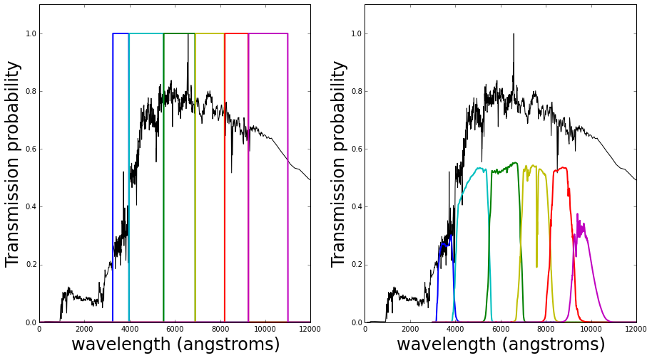
The atmosphere
For ground-based telescopes we have to observe the universe through our own atmosphere, which absorbs and scatters some of the incident light. The resulting transmission of light through our atmosphere varies depending on the quantity of different consituents during the observation (including ozone and water vapor). The quantity and distribution of these constituents varies seasonally, and also on an hourly basis.
The water vapor is one of the most interesting components because it has huge absorption effects at around 9,000 to 10,000 angstroms (angstrom=$10^{-10}$ meters). This is modelled for typical conditions and particularly evident in the wiggly-ness of the purple filter on the right.
The transmission by the purple filter can increase and decrease according to the amount of water vapor in the atmosphere. Below is a model showing the difference between two potential purple filters when there is a normal/low amount of water vapor in the atmosphere and an extreme amount.
It’s clear from these two realisations of this filter that they both probe slightly different parts of a galaxy spectrum, therefore they contain potentially different information.
In [47]:
filter_y3 = np.loadtxt('LSST_y3.dat')
filter_y4 = np.loadtxt('LSST_y.res')

fig = plt.figure(figsize=(5,5))
ax = fig.add_subplot(111)
ax.plot(filter_y3[:,0], filter_y3[:,1], linestyle='solid', color='purple', label='extreme')
ax.plot(filter_y4[:,0], filter_y4[:,1], linestyle='dashed', color='purple', label='normal')


ax.set_xlim([8000, 12000])
ax.set_ylim([0, 0.4])
ax.set_xlabel('wavelength (angstroms)', fontsize=24)
ax.set_ylabel('Transmission probability', fontsize=24)
handles, labels = ax.get_legend_handles_labels()
ax.legend(labels, loc='upper right', fontsize=16)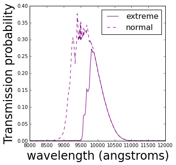
The potential information gain
I want to test if this information is retrievable given the huge diversity of galaxies (many different spectra at may different redshifts) and the measurement errors on the observed flux through this filter.
Although the two realisations of the filters are fairly different, there is a lot of ambiguity in measurements of flux through a filter. First, there are a lot of different possible spectra for galaxies: the spectrum of galaxy A through the “extreme” filter could produce the same observed flux as the spectrum of galaxy B through the “normal” filter. Because the “normal” filter covers all the same wavelengths as the “extreme” filter, and we have no way of telling what exact wavelengths the photons are at, then we can’t measure if there’s anything different between the underlying spectra from the measurements of these two galaxies. Second, galaxies are at different distances (called redshifts) and this means the further they are away the more their spectrum becomes stretched and shifted to higher wavlengths (towards the right in the previous plots). Therefore the previous scenario could be re-jigged to be the same underlying galaxy spectrum, except shifted to two different redshifts. Therefore both having different galaxy spectra, and having galaxy spectra at different redshifts, contribute to this ambiguity.
Finally the observed flux through a filter comes with some associated measurement error which can be very large for galaxies on the threshold of being detectable. This contributes some uncertainty to exactly how much flux has been observed through either of these filters.
Simulations
Let’s assume we do a large galaxy survey (like that to be done by LSST) where every galaxy will be observed hundreds of times though each of the six filters plotted above, and then all the observations are added together to create a final very precise set of six observations. We could do this survey assuming a fixed transmission by the atmosphere (really where the data is “corrected” to some fixed transmission - don’t ask how!) or we could model the individual atmospheric transmissions for each observation. In this universe let’s just assume there are only two possible atmospheric transmissions and they end up producing the “extreme” and “normal” filters above.
Then let’s simulate two galaxy surveys:
- all of the hundreds of observations per galaxy are made through all six filters shown on the right hand side in the plot above.
- all of the hundreds of observations of each galaxy are made through only the first five filters in the plot above, and then half of the observations for the last filter are made through the “extreme” filter and half through the “normal” filter. Therefore the final observations through each of the “extreme” and “normal” filters will be \( 1/\sqrt 2 \) as precise as when all of the observations are made through the “normal” filter alone (as in the first case).
In this pretend universe we will assume a galaxy can have one of 129 different possible spectra, and that there are equal numbers of each of these galaxy spectra at every redshift.
We will simulate each galaxy (each one of the galaxy spectra) 100 times at each redshift, producing different observations because of the measurement errors on the observed flux in each filter.
Redshifts will be assigned in two ways: (i) every one of these 100 galaxies will be placed at the same redshift, one out of ten redshifts overall, and (ii) each galaxy is assigned a redshift uniformly between a maximum and a minimum.
Case (i) is an overly-simplistic universe where galaxies can only exist at 10 fixed distances. This reduces the abiguity between the underlying galaxy spectrum at different redshifts and the resulting flux in a filter. It will be useful for testing.
Test 1: classifying the observation filter
If there is different information contained within the “extreme” and “normal” filters then data originating from the “extreme” filter should be separable from data originating from the “normal” filter. Here I try using a Random Forest Classifier to learn the difference between the data from the two different filters.
This is repeated four times:
- the “easy” case of having no measurement errors and data at only 10 unique redshifts. This reduces the ambiguity in the data considerably.
- a “medium” case of having no measurement errors but having data at continuous redshifts.
- another “medium” case of having measurement errors but having data at 10 unique redshifts.
- the “hard” case (which is much closer to the real universe than the others) having measurement errors and having data at continuous redshifts.
Note that the only data that goes into the classifier is the flux measured through either the “extreme” filter or the “normal” filter, and a 0 or 1 indicating which filter the data originated from. No data from the other filters (the first five) is used (yet).
In [48]:
import pandas as pd
import sklearn.ensemble as sklearn


### Data sets to read in
# Each data set contains observations for both kinds of galaxy surveys
case_i_dataset = 'brown_y3y4_photometry.txt'
case_ii_dataset = 'brown_y3y4_randz_photometry.txt'
data_sets = [case_i_dataset, case_ii_dataset, case_i_dataset, case_ii_dataset]


### Column names to read in
# For each data set first use the observations *without* measurement errors
# then use the observations *with* measurement errors
col_names = [["y_true_0", "y_true_1"], ["y_true_0", "y_true_1"],
             ["y_obs_0", "y_obs_1"], ["y_obs_0", "y_obs_1"] ]


recall = np.zeros((len(data_sets),))
precision = np.zeros((len(data_sets),))
for idata, (dset, cols) in enumerate(zip(data_sets, col_names)):

    print "Reading in data set:", dset ,"and using columns", cols


    ### Read in data
    # z=redshift, SED=spectrum type, ugrizy are the labels of each filter
    # x_true is the observation *without* the measurement error
    # x_obs is the observation *with* the measurement error
    names = ['z','SED','u_obs', 'u_err', 'u_true', 'g_obs', 'g_err', 'g_true', 'r_obs', 'r_err', 'r_true',
                   'i_obs', 'i_err', 'i_true', 'z_obs', 'z_err', 'z_true', 'y_obs', 'y_err', 'y_true']


    # the y filter is split into two for the second galaxy survey:
    ny = 2
    for i in range(ny):

        names.append('y_obs_' + str(i))
        names.append('y_err_' + str(i))
        names.append('y_true_' + str(i))


    # total number of filters
    nfilters = ny + 6
    data_types = [float] + ['S10'] + [ float for n in range(nfilters*3) ]
    df = pd.read_csv(dset, delimiter='  ', names=names, engine='python')
    print "Shape of data read in", df.shape


    ### Randomise order of data (make it easier to grab a training set later)
    df_r = df.sample(n=len(df))[cols]


    ### Create new data set consisting of JUST: y_#, filter_#
    print "Creating new data set of y filter mag vs filter class"
    nSample = len(df)*2
    y_filter_data = np.zeros((nSample, 1))
    class_y_filter = np.zeros((nSample, ))

    i = 0
    for row in df_r.iterrows():
        gal = row[1][cols]

        y_filter_data[i] = gal[0]
        class_y_filter[i] = 0
        i+=1
        y_filter_data[i] = gal[1]
        class_y_filter[i] = 1
        i+=1

    ### Random Forest
    rF = sklearn.RandomForestClassifier(n_estimators=10, criterion='gini', max_depth=None, min_samples_split=2,
                                    min_samples_leaf=1, min_weight_fraction_leaf=0.0, max_features='auto',
                                    max_leaf_nodes=None, bootstrap=True, oob_score=False, n_jobs=-1,
                                    random_state=None, verbose=0, warm_start=False, class_weight=None)


    # training sample size 80% of whole sample
    nTrain = int(round(0.8*nSample))
    print "Training sample size =", nTrain


    # fit and predict
    rF.fit(y_filter_data[:nTrain], class_y_filter[:nTrain])
    class_pred = rF.predict(y_filter_data[nTrain:])
    class_true = class_y_filter[nTrain:]


    ### Estimate recall and precision
    nTest = nSample - nTrain
    print "Testing sample size =", nTest
    num_true_positive = 0
    num_true_negative = 0
    num_false_positive = 0
    num_false_negative = 0
    for i in xrange(nTest):

        ctrue = class_true[i]
        cpred = class_pred[i]

        # if classifier got it right
        if (ctrue==cpred):

            if (ctrue>0):
                # if true class = 1 -> true positive
                num_true_positive += 1
            else:
                # if true class = 0 -> true negative
                num_true_negative += 1
        else:

            if (ctrue>0):
                # if true class = 1 -> false positive (falsely says class=1)
                num_false_positive += 1
            else:
                # if true class = 0 -> false negative (falsely says class=0)
                num_false_negative += 1

    print "True positive =", num_true_positive ,"False positive =", num_false_positive
    print "False negative =", num_false_negative ,"True negative =", num_true_negative
    print ""

    recall[idata] = num_true_positive/float(num_true_positive+num_false_negative)
    precision[idata] = num_true_positive/float(num_true_positive+num_false_positive)

    print "Recall =", recall[idata]
    print "Precision =", precision[idata], "\n"


### Plot the results!
fig = plt.figure(figsize=(20,10))
ax = fig.add_subplot(121)
ax.plot(range(len(data_sets)), recall, linestyle='solid', marker='o', color='blue', linewidth=2,
        label='recall')
ax.plot(range(len(data_sets)), precision, linestyle='dashed', marker='o', color='red', linewidth=2,
        label='precision')
ax.set_ylabel('Performance', fontsize=24, fontweight='bold')
ax.set_title('$yX$-only', fontsize=24, fontweight='bold')
handles, labels = ax.get_legend_handles_labels()
ax.legend(labels, loc='upper right', fontsize=24)
names = ['Data set 1', 'Data set 2', 'Data set 3', 'Data set 4']
plt.xticks(range(len(data_sets)), names, rotation=60, fontsize=14, fontweight='bold')
Reading in data set: brown_y3y4_photometry.txt and using columns ['y_true_0', 'y_true_1']
Shape of data read in (129000, 26)
Creating new data set of y filter mag vs filter class
Training sample size = 206400
Testing sample size = 51600
True positive = 25800 False positive = 0
False negative = 21 True negative = 25779
Recall = 0.999186708493
Precision = 1.0
Reading in data set: brown_y3y4_randz_photometry.txt and using columns ['y_true_0', 'y_true_1']
Shape of data read in (129000, 26)
Creating new data set of y filter mag vs filter class
Training sample size = 206400
Testing sample size = 51600
True positive = 12406 False positive = 13394
False negative = 12188 True negative = 13612
Recall = 0.504431975279
Precision = 0.480852713178
Reading in data set: brown_y3y4_photometry.txt and using columns ['y_obs_0', 'y_obs_1']
Shape of data read in (129000, 26)
Creating new data set of y filter mag vs filter class
Training sample size = 206400
Testing sample size = 51600
True positive = 14559 False positive = 11241
False negative = 10106 True negative = 15694
Recall = 0.590269612812
Precision = 0.564302325581
Reading in data set: brown_y3y4_randz_photometry.txt and using columns ['y_obs_0', 'y_obs_1']
Shape of data read in (129000, 26)
Creating new data set of y filter mag vs filter class
Training sample size = 206400
Testing sample size = 51600
True positive = 12344 False positive = 13456
False negative = 12135 True negative = 13665
Recall = 0.504268965236
Precision = 0.478449612403
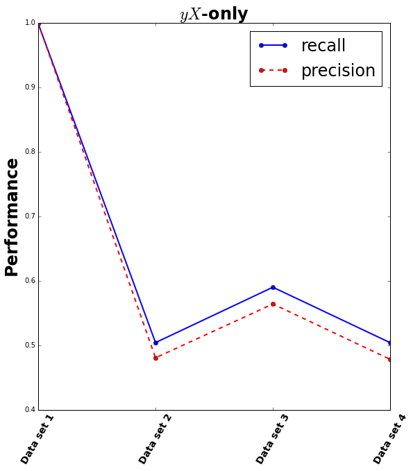
The result shows that the easy case gets near-perfect classification, but adding in any other ambiguity into the data results in a recall and precision close to 0.5: no better than guessing.
However we have extra data that can help break the ambiguity from different galaxy spectra and different redshifts: the other 5 filters! Let’s repeat with using those as well.
In [49]:
### Column names to read in
# For each data set first use the observations *without* measurement errors
# then use the observations *with* measurement errors
col_names = [['u_true','g_true','r_true','i_true','z_true',"y_true_0", "y_true_1"],
             ['u_true','g_true','r_true','i_true','z_true',"y_true_0", "y_true_1"],
             ['u_obs','g_obs','r_obs','i_obs','z_obs',"y_obs_0", "y_obs_1"],
             ['u_obs','g_obs','r_obs','i_obs','z_obs',"y_obs_0", "y_obs_1"] ]

recall = np.zeros((len(data_sets),))
precision = np.zeros((len(data_sets),))
for idata, (dset, cols) in enumerate(zip(data_sets, col_names)):

    print "Reading in data set:", dset ,"and using columns", cols


    ### Read in data
    # z=redshift, SED=spectrum type, ugrizy are the labels of each filter
    # x_true is the observation *without* the measurement error
    # x_obs is the observation *with* the measurement error
    names = ['z','SED','u_obs', 'u_err', 'u_true', 'g_obs', 'g_err', 'g_true', 'r_obs', 'r_err', 'r_true',
                   'i_obs', 'i_err', 'i_true', 'z_obs', 'z_err', 'z_true', 'y_obs', 'y_err', 'y_true']

    # the y filter is split into two for the second galaxy survey:
    ny = 2
    for i in range(ny):

        names.append('y_obs_' + str(i))
        names.append('y_err_' + str(i))
        names.append('y_true_' + str(i))


    nfilters = ny + 6
    data_types = [float] + ['S10'] + [ float for n in range(nfilters*3) ]
    df = pd.read_csv(dset, delimiter='  ', names=names, engine='python')
    print "Shape of data read in", df.shape


    ### Randomise order of data (make it easier to grab a training set later)
    df_r = df.sample(n=len(df))[cols]


    ### Create new data set consisting of now: ugriz, y_#, filter_#
    print "Creating new data set of ugriz + y filter mag vs filter class"
    nSample = len(df)*2
    filter_data = np.zeros((nSample, 6))
    class_y_filter = np.zeros((nSample, ))

    i = 0
    for row in df_r.iterrows():


        data1 = np.zeros((6,))
        data2 = np.zeros((6,))
        for ic in range(len(cols)-2):
            data1[ic] = row[1][cols[ic]]
            data2[ic] = row[1][cols[ic]]

        data1[5] = row[1][cols[5]]
        data2[5] = row[1][cols[6]]


        filter_data[i,:] = data1
        class_y_filter[i] = 0
        i+=1
        filter_data[i,:] = data2
        class_y_filter[i] = 1
        i+=1


    ### Random Forest
    rF = sklearn.RandomForestClassifier(n_estimators=10, criterion='gini', max_depth=None, min_samples_split=2,
                                    min_samples_leaf=1, min_weight_fraction_leaf=0.0, max_features='auto',
                                    max_leaf_nodes=None, bootstrap=True, oob_score=False, n_jobs=-1,
                                    random_state=None, verbose=0, warm_start=False, class_weight=None)


    # training sample size 80% of whole sample
    nTrain = int(round(0.8*nSample))
    print "Training sample size =", nTrain


    # fit and predict
    rF.fit(filter_data[:nTrain,:], class_y_filter[:nTrain])
    class_pred = rF.predict(filter_data[nTrain:,:])
    class_true = class_y_filter[nTrain:]

    nTest = nSample - nTrain
    print "Testing sample size =", nTest
    num_true_positive = 0
    num_true_negative = 0
    num_false_positive = 0
    num_false_negative = 0
    for i in xrange(nTest):

        ctrue = class_true[i]
        cpred = class_pred[i]

        # if classifier got it right
        if (ctrue==cpred):

            if (ctrue>0):
                # if true class = 1 -> true positive
                num_true_positive += 1
            else:
                # if true class = 0 -> true negative
                num_true_negative += 1
        else:

            if (ctrue>0):
                # if true class = 1 -> false positive (falsely says class=1)
                num_false_positive += 1
            else:
                # if true class = 0 -> false negative (falsely says class=0)
                num_false_negative += 1

    print "True positive =", num_true_positive ,"False positive =", num_false_positive
    print "False negative =", num_false_negative ,"True negative =", num_true_negative
    print ""

    recall[idata] = num_true_positive/float(num_true_positive+num_false_negative)
    precision[idata] = num_true_positive/float(num_true_positive+num_false_positive)

    print "Recall =", recall[idata]
    print "Precision =", precision[idata], "\n"


### Plot the results!
fig = plt.figure(figsize=(10,10))
ax = fig.add_subplot(111)
ax.plot(range(len(data_sets)), recall, linestyle='solid', marker='o', linewidth=2, color='blue',
        label='recall')
ax.plot(range(len(data_sets)), precision, linestyle='dashed', marker='o', linewidth=2, color='red',
        label='precision')
ax.set_ylabel('Performance', fontsize=24, fontweight='bold')
ax.set_title('$ugriz+yX$', fontsize=24, fontweight='bold')
handles, labels = ax.get_legend_handles_labels()
ax.legend(labels, loc='upper right', fontsize=24)
names = ['Data set 1', 'Data set 2', 'Data set 3', 'Data set 4']
plt.xticks(range(len(data_sets)), names, rotation=60, fontsize=14, fontweight='bold')
Reading in data set: brown_y3y4_photometry.txt and using columns ['u_true', 'g_true', 'r_true', 'i_true', 'z_true', 'y_true_0', 'y_true_1']
Shape of data read in (129000, 26)
Creating new data set of ugriz + y filter mag vs filter class
Training sample size = 206400
Testing sample size = 51600
True positive = 25800 False positive = 0
False negative = 0 True negative = 25800
Recall = 1.0
Precision = 1.0
Reading in data set: brown_y3y4_randz_photometry.txt and using columns ['u_true', 'g_true', 'r_true', 'i_true', 'z_true', 'y_true_0', 'y_true_1']
Shape of data read in (129000, 26)
Creating new data set of ugriz + y filter mag vs filter class
Training sample size = 206400
Testing sample size = 51600
True positive = 23252 False positive = 2548
False negative = 1284 True negative = 24516
Recall = 0.94766873166
Precision = 0.901240310078
Reading in data set: brown_y3y4_photometry.txt and using columns ['u_obs', 'g_obs', 'r_obs', 'i_obs', 'z_obs', 'y_obs_0', 'y_obs_1']
Shape of data read in (129000, 26)
Creating new data set of ugriz + y filter mag vs filter class
Training sample size = 206400
Testing sample size = 51600
True positive = 20168 False positive = 5632
False negative = 3702 True negative = 22098
Recall = 0.844909928781
Precision = 0.781705426357
Reading in data set: brown_y3y4_randz_photometry.txt and using columns ['u_obs', 'g_obs', 'r_obs', 'i_obs', 'z_obs', 'y_obs_0', 'y_obs_1']
Shape of data read in (129000, 26)
Creating new data set of ugriz + y filter mag vs filter class
Training sample size = 206400
Testing sample size = 51600
True positive = 17261 False positive = 8539
False negative = 5325 True negative = 20475
Recall = 0.764234481537
Precision = 0.669031007752
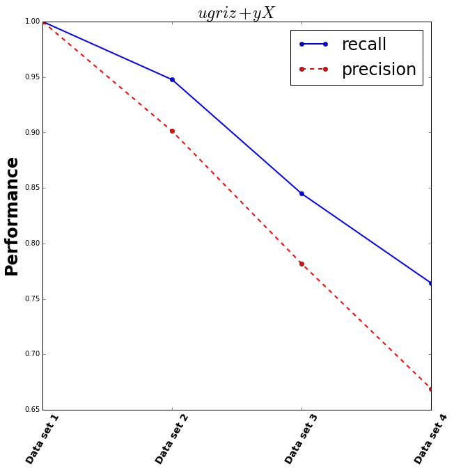
This is more hopeful! However with the recall only at around 0.75, this means only about 75% of the filters were distinguisable, and with the precision at 0.65 only 65% of the filters were correctly classed which is only slightly better than guessing. It’s not clear from this if the extra information from using both slightly different filters will help us estimate galaxy properties.
Test 2: estimating redshifts
Still, let’s see if we can use the extra information from the separate filters to learn something about the galaxy: its redshift.
Instead of classifying the data, I will use all of the data from each galaxy survey to attempt to estimate the redshift of the galaxy. I will train a Random Forest Regressor to find a mapping between the flux observed in each filter and the redshift. If splitting up the flux observations into the “extreme and “normal” filters is better than doing all the observations in the “normal” filter then the resulting redshifts will be closer to the true ones for more galaxies in that survey.
Everything below uses case (ii) with continuous redshifts.
First I try using data without measurement errors to get a maximal limit for how useful the extra information could be.
In [50]:
### Read in data
names = ['z','SED','u_obs', 'u_err', 'u_true', 'g_obs', 'g_err', 'g_true', 'r_obs', 'r_err', 'r_true',
                   'i_obs', 'i_err', 'i_true', 'z_obs', 'z_err', 'z_true', 'y_obs', 'y_err', 'y_true']

# the y filter is split into two for the second galaxy survey:
ny = 2
for i in range(ny):

    names.append('y_obs_' + str(i))
    names.append('y_err_' + str(i))
    names.append('y_true_' + str(i))


nfilters = ny + 6
data_types = [float] + ['S10'] + [ float for n in range(nfilters*3) ]
df = pd.read_csv(case_ii_dataset, delimiter='  ', names=names, engine='python')


### Columns of interest
# only the data *without* measurement errors
all_visits = ['u_true','g_true','r_true','i_true','z_true','y_true']
half_visits_y = ['u_true','g_true','r_true','i_true','z_true']
all_filters = list(all_visits)
for i in range(ny):
    half_visits_y.append('y_true_' + str(i))
    all_filters.append('y_true_' + str(i))


### Randomise order of data (make it easier to grab a training set later)
df_r = df.sample(n=len(df))[all_filters + ["z"]]


### Random Forest
rF = sklearn.RandomForestRegressor(n_estimators=10, criterion='mse', max_depth=None, min_samples_split=2,
                                   min_samples_leaf=1, min_weight_fraction_leaf=0.0, max_features='auto',
                                   max_leaf_nodes=None, bootstrap=True, oob_score=False, n_jobs=-1,
                                   random_state=None, verbose=0, warm_start=False)


# training sample size 80% of whole sample
nTrain = int(round(0.8*len(df_r)))
print "Training sample size =", nTrain


# fit all visits data
cols = all_visits
print "all visits, columns in fit are:", cols
rF.fit(df_r[cols].iloc[:nTrain], df_r["z"].iloc[:nTrain])
z_pred_all = rF.predict(df_r[cols].iloc[nTrain:])

# fit half y visits data
cols = half_visits_y
print "half visits in y, columns in fit are:", cols
rF.fit(df_r[cols].iloc[:nTrain], df_r["z"].iloc[:nTrain])
z_pred_halfy = rF.predict(df_r[cols].iloc[nTrain:])


### Bin results by true redshift
minz = 0.1
dz = 0.2
nz = 10

# true redshifts of testing sample
testing_true_z = np.asarray(df_r["z"].iloc[nTrain:])

# difference between predicted z and true z for each survey
dzp_y3y4 = np.abs(z_pred_halfy - testing_true_z)
dzp_y4 = np.abs(z_pred_all - testing_true_z)

# difference between surveys
# if positive then single filter better
# if negative then two filters better
ddzp = dzp_y3y4 - dzp_y4

frac_y3y4 = np.zeros((nz,))
frac_y4 = np.zeros((nz,))
frac_0 = np.zeros((nz,))
zc = np.zeros((nz,))
for i in range(nz):

    bl = minz + i*dz
    bh = bl + dz
    zc[i] = bl + dz/2.

    # find all galaxies in redshift bin
    idz = (testing_true_z >= bl) & (testing_true_z < bh)

    # check fraction of ddzp<0 etc
    tol = 0.001
    frac_y3y4[i] = len( np.where(ddzp[idz]<=-tol)[0]==True  )/float(len(ddzp[idz]))
    frac_y4[i] =  len(np.where(ddzp[idz]>=tol)[0]==True)/float(len(ddzp[idz]))
    frac_0[i] = len(np.where( (ddzp[idz]>-tol) & (ddzp[idz]<tol) )[0]==True)/float(len(ddzp[idz]))


fig = plt.figure(figsize=(10,10))
ax = fig.add_subplot(111)
ax.plot(zc, frac_y3y4, marker='.', linestyle='solid', color='blue', linewidth=2, label='both filters better')
ax.plot(zc, frac_y4, marker='.', linestyle='solid', color='cyan', linewidth=2, label='single filter better')
ax.plot(zc, frac_0, marker='.', linestyle='dotted', color='black', linewidth=2, label='neither better')
ax.set_xlabel('true redshift', fontsize=24, fontweight='bold')
ax.set_ylabel('fraction of galaxies where ... (see legend)', fontsize=24, fontweight='bold')
ax.set_title('no measurement errors', fontsize=24, fontweight='bold')
ax.set_ylim([-0.1, 1.1])
handles, labels = ax.get_legend_handles_labels()
ax.legend(labels, loc='upper right', fontsize=24)
Training sample size = 103200
all visits, columns in fit are: ['u_true', 'g_true', 'r_true', 'i_true', 'z_true', 'y_true']
half visits in y, columns in fit are: ['u_true', 'g_true', 'r_true', 'i_true', 'z_true', 'y_true_0', 'y_true_1']
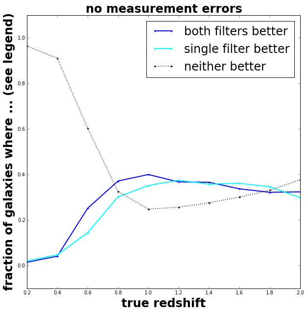
It appears that splitting up the data over two filters has a very slight improvement for galaxies closer than a redshift of 1. Probably at larger redshifts (distances) the measurement errors become too large (as the galaxies are fainter) and this masks the information.
Anyway, now we don’t expect too much for the realistic case of having data with measurement errors, but here goes.
In [51]:
### Columns of interest
# only the data *with* measurement errors
all_visits = ['u_obs','g_obs','r_obs','i_obs','z_obs','y_obs']
half_visits_y = ['u_obs','g_obs','r_obs','i_obs','z_obs']
all_filters = list(all_visits)
for i in range(ny):
    half_visits_y.append('y_obs_' + str(i))
    all_filters.append('y_obs_' + str(i))


### Randomise order of data (make it easier to grab a training set later)
df_r = df.sample(n=len(df))[all_filters + ["z"]]


### Random Forest
rF = sklearn.RandomForestRegressor(n_estimators=10, criterion='mse', max_depth=None, min_samples_split=2,
                                   min_samples_leaf=1, min_weight_fraction_leaf=0.0, max_features='auto',
                                   max_leaf_nodes=None, bootstrap=True, oob_score=False, n_jobs=-1,
                                   random_state=None, verbose=0, warm_start=False)


# training sample size 80% of whole sample
nTrain = int(round(0.8*len(df_r)))
print "Training sample size =", nTrain


# fit all visits data
cols = all_visits
print "all visits, columns in fit are:", cols
rF.fit(df_r[cols].iloc[:nTrain], df_r["z"].iloc[:nTrain])
z_pred_all = rF.predict(df_r[cols].iloc[nTrain:])

# fit half y visits data
cols = half_visits_y
print "half visits in y, columns in fit are:", cols
rF.fit(df_r[cols].iloc[:nTrain], df_r["z"].iloc[:nTrain])
z_pred_halfy = rF.predict(df_r[cols].iloc[nTrain:])


### Bin results by true redshift
minz = 0.1
dz = 0.2
nz = 10

# true redshifts of testing sample
testing_true_z = np.asarray(df_r["z"].iloc[nTrain:])

# difference between predicted z and true z for each survey
dzp_y3y4 = np.abs(z_pred_halfy - testing_true_z)
dzp_y4 = np.abs(z_pred_all - testing_true_z)

# difference between surveys
# if positive then single filter better
# if negative then two filters better
ddzp = dzp_y3y4 - dzp_y4

frac_y3y4 = np.zeros((nz,))
frac_y4 = np.zeros((nz,))
frac_0 = np.zeros((nz,))
zc = np.zeros((nz,))
for i in range(nz):

    bl = minz + i*dz
    bh = bl + dz
    zc[i] = bl + dz/2.

    # find all galaxies in redshift bin
    idz = (testing_true_z >= bl) & (testing_true_z < bh)

    # check fraction of ddzp<0 etc
    tol = 0.001
    frac_y3y4[i] = len( np.where(ddzp[idz]<=-tol)[0]==True  )/float(len(ddzp[idz]))
    frac_y4[i] =  len(np.where(ddzp[idz]>=tol)[0]==True)/float(len(ddzp[idz]))
    frac_0[i] = len(np.where( (ddzp[idz]>-tol) & (ddzp[idz]<tol) )[0]==True)/float(len(ddzp[idz]))


fig = plt.figure(figsize=(10,10))
ax = fig.add_subplot(111)
ax.plot(zc, frac_y3y4, marker='.', linestyle='solid', color='blue', linewidth=2, label='both filters better')
ax.plot(zc, frac_y4, marker='.', linestyle='solid', color='cyan', linewidth=2, label='single filter better')
ax.plot(zc, frac_0, marker='.', linestyle='dotted', color='black', linewidth=2, label='neither better')
ax.set_xlabel('true redshift', fontsize=24, fontweight='bold')
ax.set_ylabel('fraction of galaxies where ... (see legend)', fontsize=24, fontweight='bold')
ax.set_title('with measurement errors', fontsize=24, fontweight='bold')
ax.set_ylim([-0.1, 1.1])
handles, labels = ax.get_legend_handles_labels()
ax.legend(labels, loc='upper right', fontsize=24)
Training sample size = 103200
all visits, columns in fit are: ['u_obs', 'g_obs', 'r_obs', 'i_obs', 'z_obs', 'y_obs']
half visits in y, columns in fit are: ['u_obs', 'g_obs', 'r_obs', 'i_obs', 'z_obs', 'y_obs_0', 'y_obs_1']
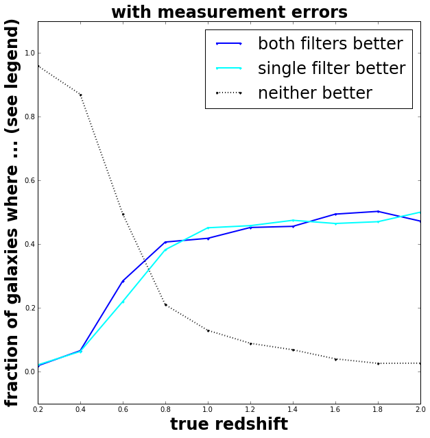
Yup, very slight improvement for galaxies at redshifts less than 0.8. The extra effort of modelling correctly multiple atmospheric transmissions probably won’t help us estimate more precise properties of galaxies.