Friends of Friends
Friends of Friends, an astronomer made clustering algorithm
The friends of friends (FoF) algorithm was first used by Huchra and Geller in 1982 to find groups of associated galaxies based upon their physical proximity. More commonly nowadays it is used to find dark matter “halos” (a system of gravitationally interacting particles that are stable, that won’t expand or collapse anymore) within a simulation of dark matter particles.
The principle is simple: two particles (or galaxies, or any discrete point in space) are grouped togther if their separation is less than some threshold, generally called the linking length. Since the distance between any two particles in a FoF group has a minimum value given by the linking length, this also acts as a density threshold.
By definition, the FoF groups cannot intersect, therefore a particle can be assigned uniquely to only one FoF group (for a single given linking length). In graph theory-speak the algorithm produces a set of connected components of an undirected graph. At the completion of the algorithm all particles are effectively “grouped”, but many may be in groups of size 1. There is also no dependence of the results on the initialisation (for a given linking length) since two particles will always be in the same group if their separation is below the threshold no matter where the algorithm began processing the data.
The runtime of the algorithm will depend not just on the implementation but also on the structure of the data. In the limiting case where all particles are within one linking length of each other the run time will be \( O(N) \). In the limiting case where no particles are within one linking length of any other particle, the run time (without optimisation) will be \( O(N^2) \); with optimisation I guess this would reduce to \( O(N\log N) \) via a divide and conquer approach.
Below is my basic implementation of the core part of this algorithm, generalised
to work in n dimensional space.
In [120]:
import numpy as np
import random
import time
from sklearn.cluster import KMeans
import matplotlib.pyplot as plt
%matplotlib inline

def group(pgroup, plist, b):
    """
        pgroup: particles already in group, list of tuples in form (id,x_i,x_j,x_k, ... x_n)
        plist:  particles not in yet group, list of tuples in form (id,x_i,x_j,x_k, ... x_n)

        where
        id is the particle id
        x_i to x_n are the coordinates of the particle in n dimensional space

        b: linking length (how close a particle needs to be to be a "friend")
    """

    # record initial lengths of lists
    ngroup = len(pgroup)
    nlist = len(plist)

    # id of everything in the group
    idg = np.array([i[0] for i in pgroup])

    # positions of everything in the group
    pg = np.array([i[1:] for i in pgroup])

    # loop over particles NOT in the group
    for p in plist:

        # particle properties
        idp = p[0] # particle id
        pp = np.array(p[1:]) # particle position

        # distance between this particle and all in the group already
        dr = np.sqrt(np.sum((pg-pp)*(pg-pp),axis=1))

        # indices of the particles with distance < b from a particle in the group
        id_in_group = np.where(dr<b)[0]

        # if there is at least one particle in the group within b of this particle
        if (len(id_in_group)>0):

            # add this particle to the group
            pgroup.append(p)
            # remove matching particle from list
            plist.remove(p)


    # check if nothing changed
    if (abs(len(pgroup)-ngroup)<0.1):
        return pgroup, plist
    else:
        return group(pgroup, plist, b)
Simulate some data
Now let’s make some data to play with. Two groups, with a Gaussian distribution of points one centered at \( (x,y)=(4,5) \) and the other at \( (x,y)=(1,2) \).
Let’s also add some sparse background of points, distributed uniformly.
In [121]:
## create list of particles with x,y positions
## they will be in two groups with x,y centers below

group1 = (4.,5.)
group2 = (1.,2.)

# number of particles in both groups
npoints = 500
# list of particles
plist = []
# groups have width 0.5, Gaussian distributed

# group 1
for i in xrange(0,npoints/2):

    x = random.gauss(group1[0],0.5)
    y = random.gauss(group1[1],0.5)
    idg = i
    plist.append((idg,x,y))

# group 2
for i in xrange(npoints/2,npoints):

    x = random.gauss(group2[0],0.5)
    y = random.gauss(group2[1],0.5)
    idg = i
    plist.append((idg,x,y))


## add some random background

# number of background particles
nback = 1000
xmin = min([i[1] for i in plist])
xmax = max([i[1] for i in plist])
ymin = min([i[2] for i in plist])
ymax = max([i[2] for i in plist])
print xmin,'< x <',xmax,ymin,'< y <',ymax
for i in xrange(npoints,npoints+nback):
    x = random.uniform(xmin,xmax)
    y = random.uniform(ymin,ymax)
    idg = i
    plist.append((idg,x,y))


# keep the original partical list
plist_orig = list(plist)
-1.32884916474 < x < 5.44355794973 0.270660525779 < y < 6.44284078467
Visualise the data
In [122]:
# list comprehension for easy extraction
xvals = [p[1] for p in plist]
yvals = [p[2] for p in plist]

# plot the points
fig = plt.figure(figsize=(10,10))
ax = fig.add_subplot(111)
ax.plot(xvals, yvals, linestyle='none', marker='.')
ax.set_xlabel('x', fontsize=24, fontweight=2)
ax.set_ylabel('y', fontsize=24, fontweight=2)

# plot the group centers
ax.plot(group1[0], group1[1], linestyle='none', marker='o', color='black', markersize=15., linewidth=5.)
ax.plot(group2[0], group2[1], linestyle='none', marker='o', color='black', markersize=15., linewidth=5.)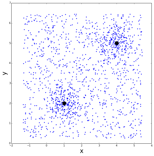
Run FoF!
In [123]:
## Run friends-of-friends

# linking length
b = 0.125

# final list of groups
groups = []

t1 = time.time()
while len(plist)>0:

    # initialize by adding the first particle in the current list into it's own "group"
    pgroup = [plist[0]]
    plist.remove(pgroup[0])

    # here's the meat:
    # find everything in plist that is within b of anything in pgroup
    # add it to pgroup, delete it from plist
    # continue (via) recursion until no more particles in plist move into pgroup
    new_group, plist = group(pgroup, plist, b)

    # add the finished group to the list
    groups.append(new_group)

print 'Found', len(groups) ,'groups from', npoints + nback ,'particles'
t2 = time.time()
print 'Time taken',t2-t1,'s'
Found 499 groups from 1500 particles
Time taken 9.47667312622 s
Results
Lets pull out the two largest groups and see if they correspond to the original groups
In [124]:
# compute size of each group
group_size = [len(g) for g in groups]

# sort by ascending group size
isort = sorted(range(len(group_size)), key=lambda k: group_size[k])

print "The largest group has", group_size[isort[-1]] ,"members"
print "The second largest group has", group_size[isort[-2]] ,"members"
print "The third largest group has", group_size[isort[-3]] ,"members"
The largest group has 236 members
The second largest group has 160 members
The third largest group has 48 members
We can see from this that it is likely the FoF algorithm found the two groups.
In [125]:
# plot the points
fig = plt.figure(figsize=(10,10))
ax = fig.add_subplot(111)
ax.plot(xvals, yvals, linestyle='none', marker='.')
ax.set_xlabel('x', fontsize=24, fontweight=2)
ax.set_ylabel('y', fontsize=24, fontweight=2)
ax.set_title('linking length, b ='  + str(b), fontsize=24, fontweight=2)

# plot the group centers
ax.plot(group1[0], group1[1], linestyle='none', marker='o',
        color='black', markersize=15., linewidth=5., label='true center')
ax.plot(group2[0], group2[1], linestyle='none', marker='o',
        color='black', markersize=15., linewidth=5.)

# plot the members of the two largest groups
xg = [p[1] for p in groups[isort[-1]] ]
yg = [p[2] for p in groups[isort[-1]] ]
mean_x1 = np.mean(xg)
mean_y1 = np.mean(yg)
ax.plot(xg, yg, linestyle='none', marker='.', color='red', markersize=5., linewidth=5.)
xg = [p[1] for p in groups[isort[-2]] ]
yg = [p[2] for p in groups[isort[-2]] ]
mean_x2 = np.mean(xg)
mean_y2 = np.mean(yg)
ax.plot(xg, yg, linestyle='none', marker='.', color='red', markersize=5., linewidth=5.)

# plot the mean x and y values in each group
ax.plot(mean_x1, mean_y1, linestyle='none', marker='*', color='purple',
        markersize=30., linewidth=5., label='FoF center')
ax.plot(mean_x2, mean_y2, linestyle='none', marker='*', color='purple',
        markersize=30., linewidth=5.)

handles, labels = ax.get_legend_handles_labels()
ax.legend(handles, labels, loc='upper left')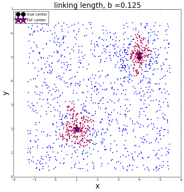
Change the linking length
Now let’s re-run with a larger linking length
In [126]:
## Run friends-of-friends
plist = list(plist_orig)

# linking length
b = 0.2

# final list of groups
groups = []

i=0
t1 = time.time()
while len(plist)>0:

    # initialize by adding the first particle in the current list into it's own "group"
    pgroup = [plist[0]]
    plist.remove(pgroup[0])

    # here's the meat:
    # find everything in plist that is within b of anything in pgroup
    # add it to pgroup, delete it from plist
    # continue (via recursion) until no more particles in plist move into pgroup
    new_group, plist = group(pgroup, plist, b)

    # add the finished group to the list
    groups.append(new_group)
    i+=1

print 'Found', len(groups) ,'groups from', npoints + nback ,'particles'
t2 = time.time()
print 'Time taken',t2-t1,'s\n'

# compute size of each group
group_size = [len(g) for g in groups]

# sort by ascending group size
isort = sorted(range(len(group_size)), key=lambda k: group_size[k])

print "The largest group has", group_size[isort[-1]] ,"members"
print "The second largest group has", group_size[isort[-2]] ,"members"
print "The third largest group has", group_size[isort[-3]] ,"members"

# plot the points
fig = plt.figure(figsize=(10,10))
ax = fig.add_subplot(111)
ax.plot(xvals, yvals, linestyle='none', marker='.')
ax.set_xlabel('x', fontsize=24, fontweight=2)
ax.set_ylabel('y', fontsize=24, fontweight=2)
ax.set_title('larger linking length, b ='  + str(b), fontsize=24, fontweight=2)

# plot the group centers
ax.plot(group1[0], group1[1], linestyle='none', marker='o',
        color='black', markersize=15., linewidth=5., label='true center')
ax.plot(group2[0], group2[1], linestyle='none', marker='o',
        color='black', markersize=15., linewidth=5.)

# plot the members of the two largest groups
xg = [p[1] for p in groups[isort[-1]] ]
yg = [p[2] for p in groups[isort[-1]] ]
mean_x1 = np.mean(xg)
mean_y1 = np.mean(yg)
ax.plot(xg, yg, linestyle='none', marker='.', color='red', markersize=5., linewidth=5.)
xg = [p[1] for p in groups[isort[-2]] ]
yg = [p[2] for p in groups[isort[-2]] ]
mean_x2 = np.mean(xg)
mean_y2 = np.mean(yg)
ax.plot(xg, yg, linestyle='none', marker='.', color='red', markersize=5., linewidth=5.)

# plot the mean x and y values in each group
ax.plot(mean_x1, mean_y1, linestyle='none', marker='*', color='purple',
        markersize=30., linewidth=5., label='FoF center')
ax.plot(mean_x2, mean_y2, linestyle='none', marker='*', color='purple',
        markersize=30., linewidth=5.)

handles, labels = ax.get_legend_handles_labels()
ax.legend(handles, labels, loc='upper left')
Found 121 groups from 1500 particles
Time taken 3.08288502693 s
The largest group has 491 members
The second largest group has 380 members
The third largest group has 46 members
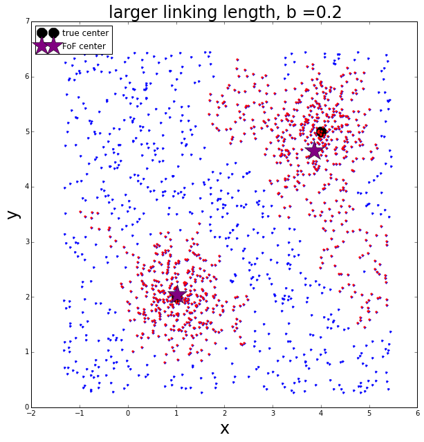
The larger linking length allows more points to be included in the two largest groups. The points appear to definitely include erroneous background points that cause the center of each group to become biased.
K-means
For fun, let’s see what the k-means clustering algorithm does.
In [127]:
# kmeans
km = KMeans(n_clusters=2, init='random', n_init=100, max_iter=300, tol=0.0001,
            precompute_distances='auto', verbose=0, random_state=None, copy_x=True, n_jobs=-1)

# convert particle tuple list into np array of just x,y positions
xy = np.asarray([(p[1],p[2]) for p in plist_orig])

# perform kmeans clustering
km.fit(xy)

# get the results
cluster_centers = km.cluster_centers_
cluster_labels = km.labels_


# plot the original points
fig = plt.figure(figsize=(10,10))
ax = fig.add_subplot(111)
ax.plot(xvals, yvals, linestyle='none', marker='.')
ax.set_xlabel('x', fontsize=24, fontweight=2)
ax.set_ylabel('y', fontsize=24, fontweight=2)

# plot the true group centers
ax.plot(group1[0], group1[1], linestyle='none', marker='o', color='black',
        markersize=15., linewidth=5., label='true center')
ax.plot(group2[0], group2[1], linestyle='none', marker='o', color='black',
        markersize=15., linewidth=5.)

# plot the kmeans cluster centers
ax.plot(cluster_centers[0,0], cluster_centers[0,1], linestyle='none', marker='*',
        color='red', markersize=30., linewidth=5.j, label='kmeans center')
ax.plot(cluster_centers[1,0], cluster_centers[1,1], linestyle='none', marker='*',
        color='red', markersize=30., linewidth=5.)

handles, labels = ax.get_legend_handles_labels()
ax.legend(handles, labels, loc='upper left')


# plot the points by kmeans cluster membership
fig = plt.figure(figsize=(10,10))
ax = fig.add_subplot(111)


cl1 = xy[np.where(cluster_labels>0)[0]]
cl2 = xy[np.where(cluster_labels<1)[0]]


ax.plot(cl1[:,0], cl1[:,1],
        linestyle='none', marker='o', color='red', label='cluster 1')
ax.plot(cl2[:,0], cl2[:,1],
        linestyle='none', marker='o', color='DarkRed', label='cluster 2')

ax.set_xlabel('x', fontsize=24, fontweight=2)
ax.set_ylabel('y', fontsize=24, fontweight=2)

handles, labels = ax.get_legend_handles_labels()
ax.legend(handles, labels, loc='upper left')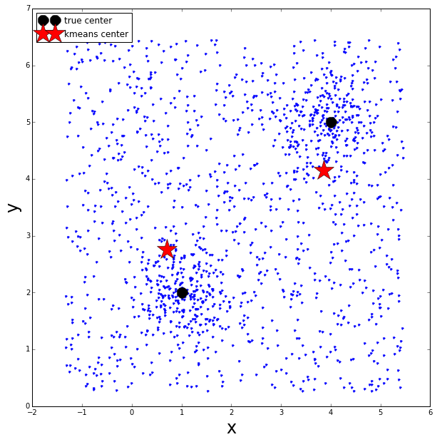
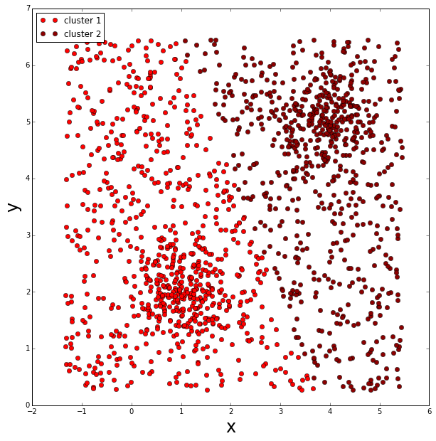
As well as having to know a priori the number of clusters we are searching for, k-means also has to assign all points into one of the pre-defined clusters, therefore this produces a significant bias in the calculated cluster centers.