Random forests and noisy data
Random forests and noisy data
I want to test how random forests deal with noisy data that has the same information content as less noisy data.
The test for this will be to see how well the random forest regressor can predict the mean of the Gaussian that the data was drawn from.
The whole data set will be drawn from a set of Gaussians with different means (\( \mu \)) but identical standard deviations (\( \sigma \)), and the following three data sets will be created:
- the data is drawn from each Gaussian ONE time. This will be termed the high noise data set, where each data point has error=\( \sigma \)
- the data is drawn from each Gaussian \( n_{obs} \) times and then averaged to produce one data point for each Gaussian. This will be termed the low noise data set, where each data point has error=\( \sigma/\sqrt(n_{obs}) \)
- the data is drawn from each Gaussian \( n_{obs} \) times but not averaged, just kept. This data set will therefore be \( n_{obs} \) times larger than data sets 1. and 2.. This will be termed the high noise-many data set, where each data point has error=\( \sigma \) but the data set contains more information due to the larger number of “observations” per Gaussian.
The data sets will be drawn from Gaussians that have means that are evenly spaced between \( \mu_{min} \) and \( \mu_{max} \). These means will be fixed over all realisations of the data sets. The spacing between \( \mu \)’s will be set equal \( \sigma \) so there is significant overlap between data drawn from adjacent Gaussians making it non-trivial for a single data point to predict the mean of the Gaussian it was drawn from.
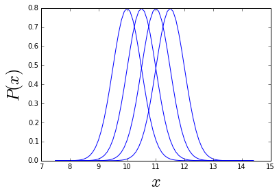
To illustrate how this might work I plot an example of 4 Gaussians spaced between \( \mu_{min}=10 \) and \( \mu_{max}=12 \) by \( \sigma=0.5 \).
In [50]:
import numpy as np
import matplotlib.pyplot as plt
import sklearn.ensemble as sklearn
%matplotlib inline

sigma = 0.5

mu_min = 10.
mu_max = 12.
mu_s = np.arange(mu_min, mu_max, sigma)

xvals = np.arange(mu_min-5.*sigma, mu_max+5.*sigma, sigma/5.)
fig = plt.figure()
ax = fig.add_subplot(111)
for mu in mu_s:

    # Gaussian with mean=mu and std=sigma
    g = 1./np.sqrt(2.*np.pi*sigma**2)*np.exp(-0.5*(xvals-mu)**2/sigma**2)
    ax.plot(xvals, g, color='blue')

ax.set_xlabel('$x$', fontsize=24)
ax.set_ylabel('$P(x)$', fontsize=24)
Now to illustrate the drawing of the different data sets, I’ll draw data points from the 4 Gaussians plotted above, with only 5 “observations” for data sets 2. and 3.
In [51]:
ntotal = len(mu_s)
print "There are", ntotal ,"Gaussians", "\n"

n_obs = 5  # 5 observations

x_high_noise = np.zeros((ntotal,1))           # data set (1)
x_low_noise  = np.zeros((ntotal,1))           # data set (2)
x_high_noise_many = np.zeros((ntotal, n_obs)) # data set (3)

for i, mu_i in enumerate(mu_s):

    # generate high noise data for data set (1)
    x_high_noise[i,0] = sigma*np.random.randn() + mu_i

    # generate low noise data for data set (2) by averaging over nobs observations
    # generate high noise-many for data set (3) by keeping all of data set (2)'s single observations
    x = 0.
    for j in xrange(n_obs):

        # generate "observation"
        xgen = sigma*np.random.randn() + mu_i

        # sum observations ready for average for data set (2)
        x += xgen

        # keep each individual observation for data set (3)
        x_high_noise_many[i,j] = xgen


    # final average for data set (2)
    x_low_noise[i,0] = x/float(n_obs)

print "The Gaussian mu's:"
print mu_s, "\n"

print "The high noise data:"
print x_high_noise, "\n"

print "The low noise data:"
print x_low_noise, "\n"

print "The high noise-many data:"
print x_high_noise_many
print "Taking the mean should retrieve the 'low noise' data:"
print np.mean(x_high_noise_many, axis=1), "\n"
There are 4 Gaussians
The Gaussian mu's:
[ 10. 10.5 11. 11.5]
The high noise data:
[[ 9.3879663 ]
[ 10.61671429]
[ 10.94476015]
[ 11.60133208]]
The low noise data:
[[ 10.342395 ]
[ 10.15318336]
[ 10.89082949]
[ 11.50473817]]
The high noise-many data:
[[ 10.83025991 10.03411825 9.58813345 11.07049289 10.18897049]
[ 10.05478904 10.54668392 9.93534111 9.68767715 10.54142557]
[ 11.80355274 10.96345827 10.06984289 10.85218006 10.7651135 ]
[ 11.63320311 11.59479556 11.21628922 11.73834815 11.34105479]]
Taking the mean should retrieve the 'low noise' data:
[ 10.342395 10.15318336 10.89082949 11.50473817]
Probably (depending on the random realisation you get!) you can see that the “high noise” data set is noiser than the “low noise” data set, and that the “high noise-many” data set columns look more like 5 different versions of the “high noise” data set that the “low noise” data set.
Anyway, now I’m going to repeat the above but with new (more illustrative) parameters for the Gaussian and generate a larger data set. Then perform random forest regression on the generated data to try and predict the mean of the Gaussian it was drawn from. For each realisation of the data sets the rms precision with which the random forest regressor found the mean of the Gaussians will be recorded.
Depending on the value of nreal this may take a few minutes to run.
In [52]:
# decreasing sigma
sigma = 0.01

# changing range of mu's
mu_min = 10.
mu_max = 100.
mu_s = np.arange(mu_min, mu_max, sigma)

ntotal = len(mu_s)
print "There are now", ntotal ,"Gaussians", "\n"

# increase number of observations
n_obs = 100

# number of times to perform experiment
nreal = 30

# final results will be stored here
rms_high_noise = np.zeros((nreal,))
rms_low_noise = np.zeros((nreal,))
rms_high_noise_many = np.zeros((nreal,))

for ireal in xrange(nreal):

    if (ireal%10==0):
        print "On realisation", ireal+1 ,"of", nreal
    np.random.shuffle(mu_s)  # shuffle so can split into training and test easily
                              # also shuffle here so training and test sets are different each realisation

    x_high_noise = np.zeros((ntotal,1))           # data set (1)
    x_low_noise  = np.zeros((ntotal,1))           # data set (2)
    x_high_noise_many = np.zeros((ntotal, n_obs)) # data set (3)

    for i, mu_i in enumerate(mu_s):

        # generate high noise data for data set (1)
        x_high_noise[i,0] = sigma*np.random.randn() + mu_i

        # generate low noise data for data set (2) by averaging over nobs observations
        # generate high noise-many for data set (3) by keeping all of data set (2)'s single observations
        x = 0.
        for j in xrange(n_obs):

            # generate "observation"
            xgen = sigma*np.random.randn() + mu_i

            # sum observations ready for average for data set (2)
            x += xgen

            # keep each individual observation for data set (3)
            x_high_noise_many[i,j] = xgen


        # final average for data set (2)
        x_low_noise[i,0] = x/float(n_obs)


    ### Random forest training and prediction
    rF = sklearn.RandomForestRegressor(n_estimators=10, criterion='mse', max_depth=None, min_samples_split=2,
                                   min_samples_leaf=1, min_weight_fraction_leaf=0.0, max_features='auto',
                                   max_leaf_nodes=None, bootstrap=True, oob_score=False, n_jobs=-1,
                                   random_state=None, verbose=0, warm_start=False)


    # split in half to train
    nTrain = int(ntotal/2.)

    # train high noise: data set (1)
    rF.fit(x_high_noise[:nTrain], mu_s[:nTrain])
    mu_pred_high_noise = rF.predict(x_high_noise[nTrain:])

    # train low noise: data set (2)
    rF.fit(x_low_noise[:nTrain], mu_s[:nTrain])
    mu_pred_low_noise = rF.predict(x_low_noise[nTrain:])

    # train high noise-many: data set (3)
    rF.fit(x_high_noise_many[:nTrain], mu_s[:nTrain])
    mu_pred_high_noise_many = rF.predict(x_high_noise_many[nTrain:])


    ### Store mean precision statistics

    # take out test sample of true y's
    mutest = mu_s[nTrain:]

    # root mean square fractional difference between predicted mu and true mu
    rms_high_noise[ireal] = np.sqrt(np.mean((mutest-mu_pred_high_noise)**2/mutest**2))
    rms_low_noise[ireal] = np.sqrt(np.mean((mutest-mu_pred_low_noise)**2/mutest**2))
    rms_high_noise_many[ireal] = np.sqrt(np.mean((mutest-mu_pred_high_noise_many)**2/mutest**2))


### Plot!
fig = plt.figure(figsize=(10,10))
ax = fig.add_subplot(111)
ax.hist(rms_high_noise, normed=True, histtype='stepfilled', color='r', label='high noise')
ax.hist(rms_low_noise, normed=True, histtype='stepfilled', color='b', label='low noise')
ax.hist(rms_high_noise_many, normed=True, histtype='stepfilled', color='r', alpha=0.5, hatch='*',
        label='high noise/many')
ax.set_xlabel('RMS fractional deviation', fontsize=24)
ax.set_title(str(nreal) + " realisations", fontsize=24)
handles, labels = ax.get_legend_handles_labels()
ax.legend(labels, loc='upper right')
There are now 9000 Gaussians
On realisation 1 of 30
On realisation 11 of 30
On realisation 21 of 30

Results!
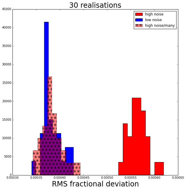
The plot above shows a histogram for each data set of the rms precision of the random forest regressor in predicting the value of the mean of each Gaussian.
The random forest run on the “high noise-many” data set turns out to be just as accurate as the one run on the “low noise” data set (and of course then also more accurate than the “high noise” data set) as we expected and hoped from our knowledge of all the statistics.